Background
Recently, I have discovered the Second Language Acquisition Modeling (SLAM) challenge hosted by Duolingo earlier this year, where they had asked the participants to predict the per-token error rate for a given language learner based on his/her past learning history. To conclude the competition, the team has also written a paper to summarize the results and the approaches that were taken by the various participants and their respective effectiveness. After reading the paper and the top competitors’ system papers (particularly the one published by SanaLabs), I just couldn’t resist playing around with the data myself :)
Given that the competition has long ended and that I have already read the system papers (and thus have the benefit of hindsight), my goal for this project is not to compete but rather to see whether, built upon the shared knowledge and experience, I can create a simple model that produces decent results. Simplicity is important because 1) I’m always curious to see how far an easily built and understandable model can go and 2) as a side project, I didn’t plan to allocate too much time to it. The goal influenced many modeling decisions. For example, instead of building three separate models, one for each track (English, Spanish, and French), I decided to build only one single shared-track model to predict the error rate for all of them in one shot. That said, I did opt directly to using an RNN instead of experimenting with a classical approach. The decision was made because I was curious to see how RNNs can be applied to the various types of sequential data with minimum feature engineering and that the team’s meta study found that using a RNN-based structure provides the biggest uplift to the final performance.
In the end, I was rather happy with my model results. In particular, the model scored the following ROC and F1 scores in the three respective tracks, which stands around the middle of all 15 participants:
All my code is hosted in this repo. The rest of the post would focus on the feature selections, the model architecture, and the post-modeling evaluations.
Features
To keep it simple, I only used the features provided in the original dataset and did not engineer anything extra myself. In particular, this means that my model includes the following user and word specific features:
- User features:
- Track (i.e.,
en_es,es_en,fr_en) - User ID
- Country1
- Client (i.e.,
ios,android,web) - Days in course
- Track (i.e.,
- Word features:
- Word2
- Part of speech
- Dependency labels
- Dependency edges
- Morphology features
- Response time
- Format (i.e.,
reverse_translate,reverse_tap,listen) - Session (i.e.,
lesson,practice,test)
The label is the per-word accuracy: 0 if correct and 1 if not.
Model
The model architecture is shown in the diagram below. Simply put, it is a bidirectional GRU model where each input is a concatenation of all the features mentioned above and each output is the predicted error rate for the current word.
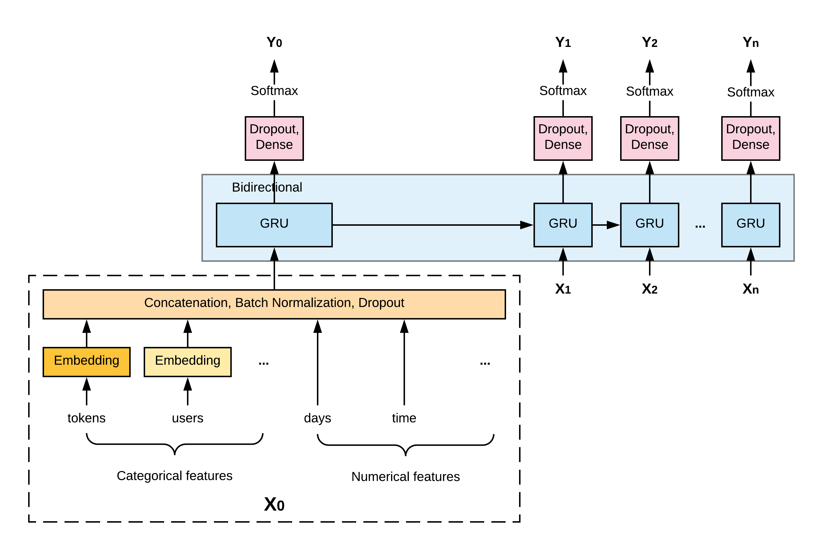
For categorical features, each of them is first mapped into a randomly-initiated embedding vector before being concatenated with the others. The embedding size is determined based on the feature’s original cardinality (in particular, cardinality // 2 3), capped at 256.
For numerical features, they are concatenated directly with the others without any preprocessing. Because of the various ranges of the input features, a batch normalization layer is added after the concatenation to speed up the training.
The bidirectional GRU has a single layer with a hidden units size of 256 (I have experimented with 2 layers but did not see an improvement in the results). I have also tried replacing GRU with LSTM, which took longer to train but only provided less than 1% of relative uplift in the results, so I stuck with GRU.
From each GRU unit, its output is further processed by two dense layers and finally a softmax activation to normalize the output into probabilities. Softmax is used instead of sigmoid, which is usually a choice for binary predictions, because aside from the original two classes, I also added an extra one for the padding token, which is necessary for batch processing.
Training
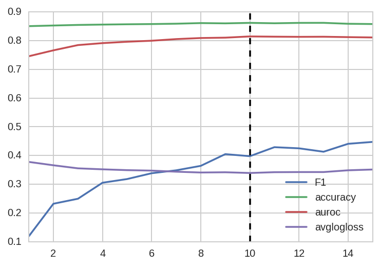
To train the model, I used the standard Adam optimizer with a learning rate of 0.001 and the cross-entropy loss. The model is trained with early stopping and, as shown below, the validation loss plateaued (and the ROC peaked) at the 10th epoch:
Finally, to take advantage of the dev data, I trained another model using the combined data under the same architecture and hyperparameters also for 10 epochs.4 The resulting model was later applied to the test data to generate final predictions.
Performance evaluation
In addition to the test set performance metrics shown above, I was also curious about the feature importance, the interpretability of the learned embeddings, and the error analysis, all of which I explored below.
Feature importance
To estimate the feature importance, I use the actual model performance on the dev set as the baseline, and shuffle one feature from the dataset at a time to measure the decrease in performance, which is then used as an indicator to the given feature’s relative importance.5 The resulting importance, in terms of both the decrease in ROC and F1 score, is shown below:
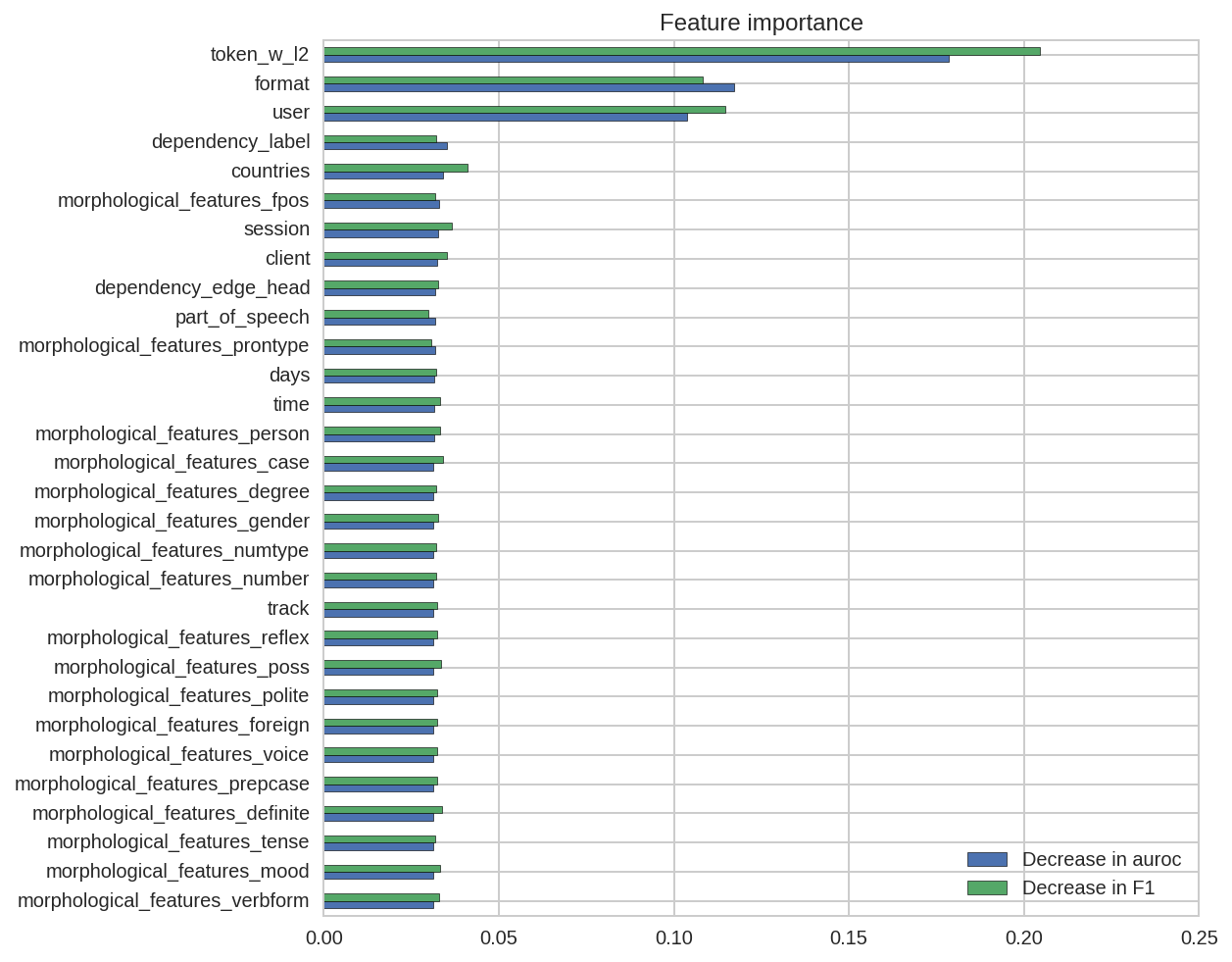
As shown above, three features stand out as the most important ones: the word itself, the exercise format, and the user.6 Among them, format is the most straightforward to understand because, compared to reverse_translate and listen, reverse_tap is much easier given that the candidate words have all been shown to the students. In fact, based on the training data, its error rate is three times less than the other two formats. As for the word and the user, they are both of high dimensions so to facilitate the interpretations, I visualized their learned embeddings below.
Learned embeddings
To visualize the high-dimensional embeddings (256), I used t-SNE combined with PCA.7 Below is the reduced 2D embeddings for all the 6K in-vocabulary words, colored by their respective per-word error rate:
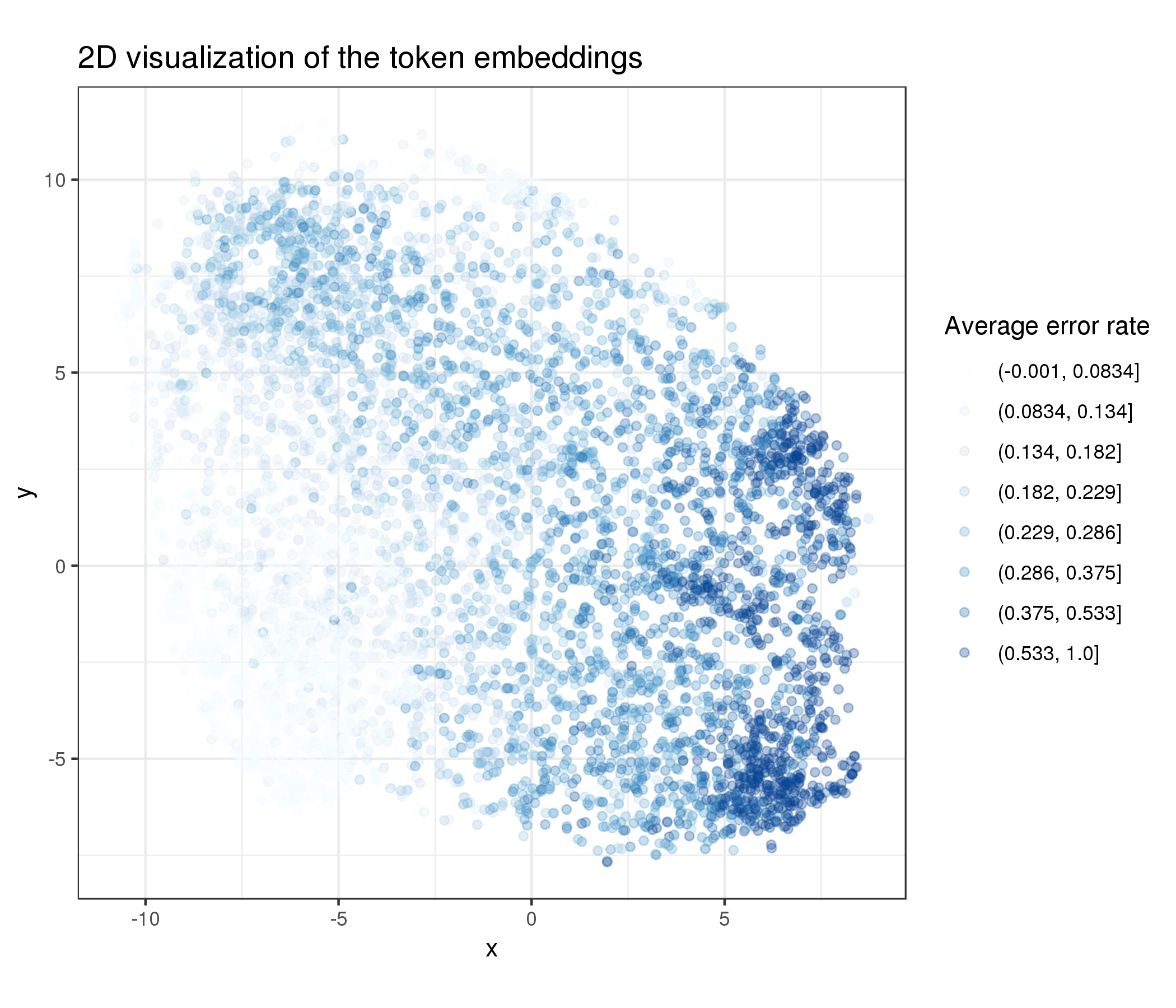
As shown above, the model appeared to have moved words with high error rates close to each other in the embedding space to make the prediction easier (i.e., the dark blue cluster in the bottom right corner). It should be noted that many of these are also low frequency words which not many students have attempted yet (and are hence presumably more difficult).
In addition, below is the same plot for all the 6K users and their average error rate:
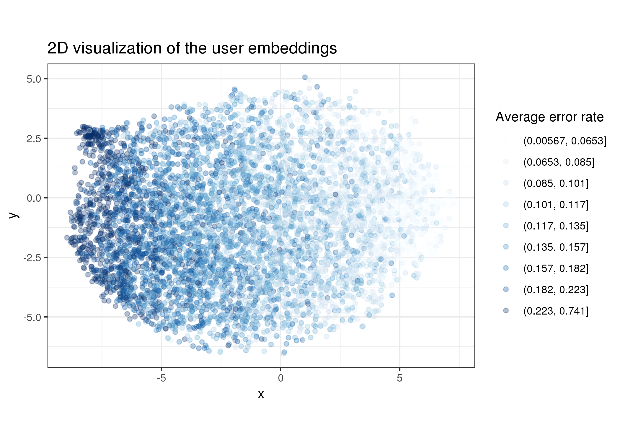
In a similar pattern as seen above, the model effectively clustered users based on their historical error rate, which is a reasonable thing to do as well.
In addition to these embeddings’ relationships with the outcome variable, I was also interested in seeing how they interact with each other. For example, do these word embeddings, trained for a specific downstream task, exhibit the same kind of pattern as those trained in an unsupervised way do (e.g., word2vec) where semantically similar words are clustered together? To answer this question, I first plotted the top 100 learned English word embeddings below:
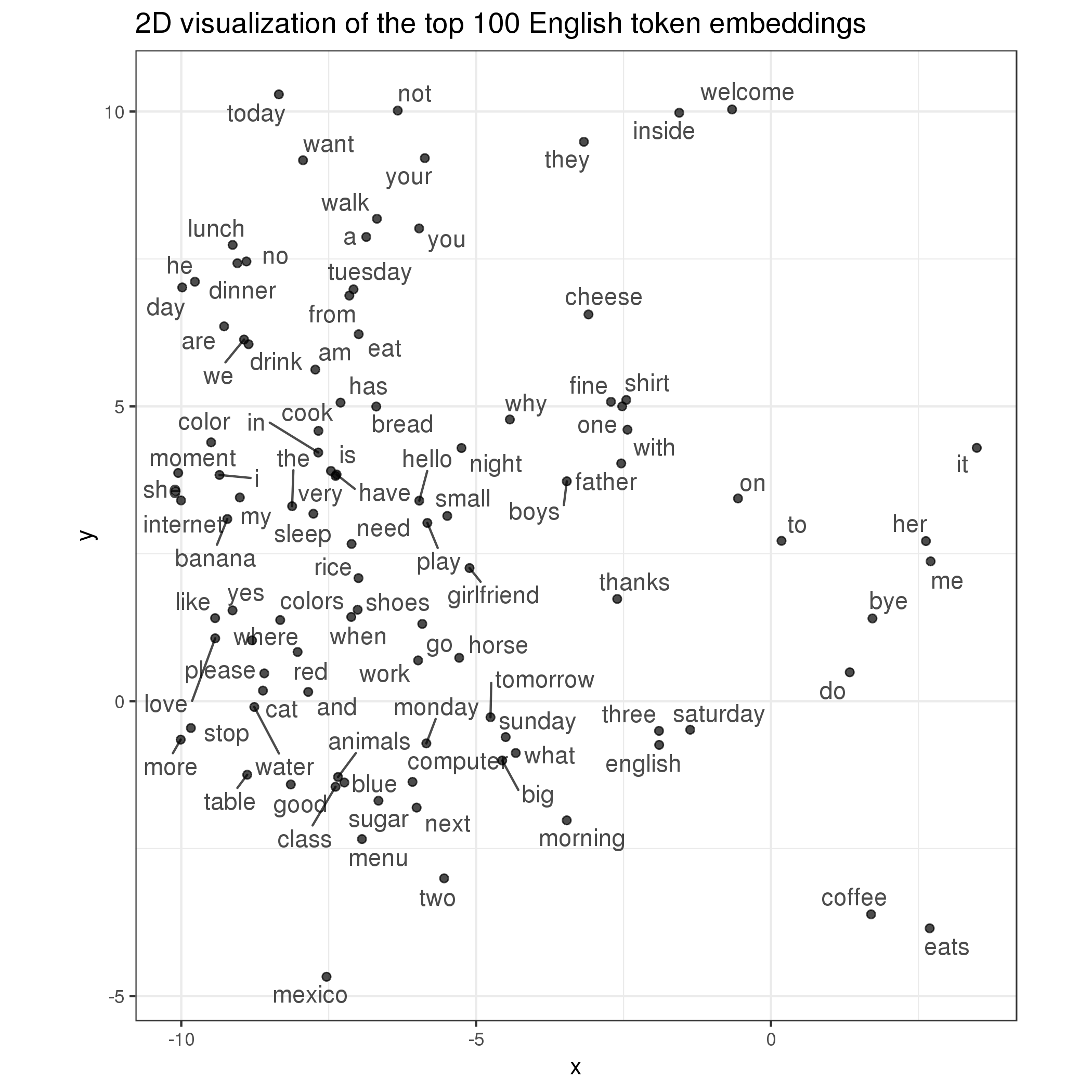
As it turns out, some of them indeed do! For example, object pronouns her, me, and it are close to each other (far-right), food-related words lunch, dinner, drink, eat, and cook are grouped together (upper-left), and time-related notions monday, sunday, saturday, tomorrow, and morning are also close (center-bottom). Why do they do this? I think one explanation is that semantically similar words are often organized into a single course and taught together based on its meanings and difficulties. Hence, students who were learning these new concepts are likely to exhibit the same level of error rate on all of them too, which led the model to push them close to each other. It also helps that the corpus includes only new learners in their first 30 days so that the learning materials conveniently overlap with each other.
At this point I had a crazy idea: trained this way, would the same words in different languages are also close to each other in the embedding space? To test this hypothesis, I plotted the top English and French word embeddings below:
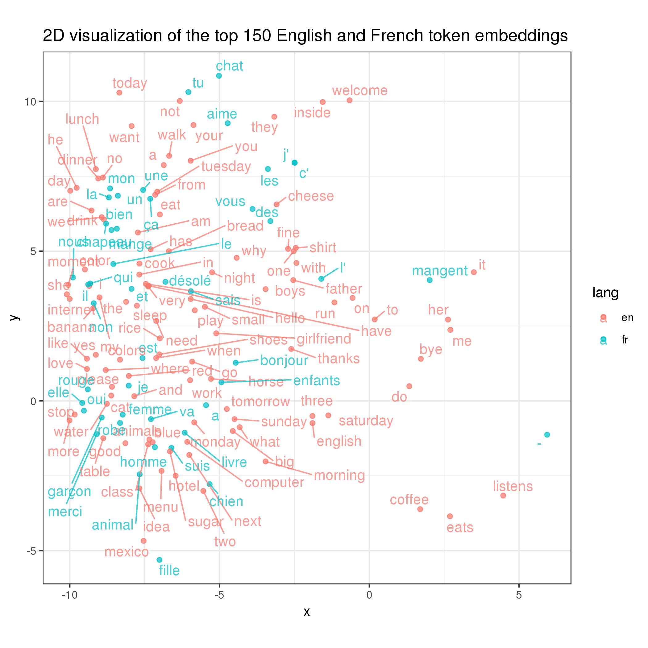
Sadly (but expectedly), it’s not quite the case as the nearby red and blue words above are rather random (despite some happy surprises like you and tu). It makes sense in the hindsight because, to make them overlap, the English and French course materials need to overlap each other too, which is not necessarily the case (although there may be similarities).
Error analysis
Lastly, I decided to do some error analysis to find out the cases where the model works well and those where it does not. In particular, I was interested in looking at it on a per-user basis because it’s the most actionable. Hence, inspired by the meta-study, I computed per-user ROC on the test set8 and my goal is to find out what factors lead to a higher or lower ROC for a given user.
My candidate explanatory variables are historical data we have for each user in the training and dev sets. In particular, I considered the following:
- Historical usage frequency (i.e., the number of words a user has attempted in the training and dev data)
- Of all the historical words a user has attempted, the % of them that are of high frequency in the corpus (i.e., the top 10% of the most common words)
- Historical error rate
- Learning track
- Client
To find out which ones of them influence the per-user ROC the most, I ran a simple linear regression controlling for all of them and found the following results:
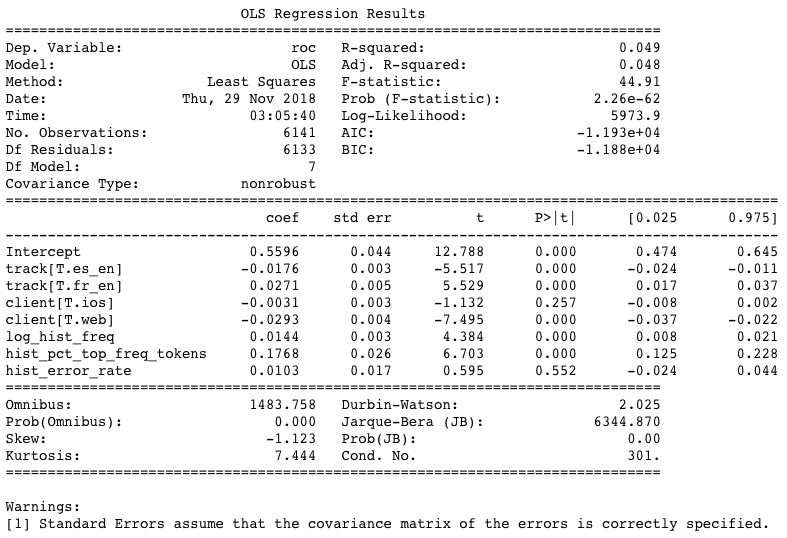
As shown above, the result suggests that:
- As expected, the model does well if a user has a lot of historical data (hence the historical frequency is positively significant and the web client is negatively so9) and if many of these historical words are also high-frequency words. Both of these findings make sense given that both words and user IDs are significant features in the model itself.
- Track also matters. In particular, on a per-user basis, the model performs the best on the
fr_entrack and the worst on thees_entrack.10 - One’s historical error rate doesn’t matter to the model’s performance on him/her, which is reassuring.
Conclusions and future work
In this project, I analyzed Duolingo’s SLAM challenge data and, upon reviewing the system papers, built an RNN-based model myself to predict the per-user, per-token error rate that yielded decent performance. Further analysis revealed that the words’ surface forms, the exercise format, and the user IDs are the most important features in the model. In addition to modeling, I have also analyzed the learned embeddings of the words and the users, which showed that the model effectively clustered them based on their respective error rates. Finally, I performed an error analysis which showed that, on a per-user basis, one’s historical usage frequency, the frequency of the words learned, as well as one’s client and track significantly correlate with the model’s performance on him/her.
There is still a lot of interesting things we can do with the data itself. One thing that I’m particularly interested in is to visualize whether and how one learns from his/her past mistakes, and how that compares with the model predictions. For example, a simplistic model that naively predicts error rate based on the past may keep predicting a user would always make the same mistake over and over again in the future, but one that takes into account of the learning trajectory may be able to adjust the error rate accordingly. Frankly, at this point, I have no idea if my model is able to do that. (If not, there would be no point in using an RNN.) I tried to sample a few users to see if there are some easy patterns but the data is too noisy. In the future, I’ll explore devising some aggregated metrics, like the actual vs. predicted conditional error rate, to see if there is a mismatch between the reality and the prediction.
References
Burr Settles, Chris Brust, Erin Gustafson, Masato Hagiwara, Nitin Madnani. Second Language Acquisition Modeling. Proceedings of the Thirteenth Workshop on Innovative Use of NLP for Building Educational Applications, pages 56–65. June 5, 2018.
Anton Osika, Susanna Nilsson, Andrii Sydorchuk, Faruk Sahin, Anders Huss. Second Language Acquisition Modeling: An Ensemble Approach. Proceedings of the Thirteenth Workshop on Innovative Use of NLP for Building Educational Applications, pages 217–222. June 5, 2018.
If a user has used Duolingo in two countries, only the first is used.↩
Because the model includes all three languages, to prevent the confusion that is resulted from the identically spelled but semantically different words, each word is concatenated with its respective language (e.g.,
en:hello).↩A rule of thumb I picked up from the fast.ai course.↩
Due to time constraint, I did not perform any hyperparameter tuning.↩
The shuffle is done on the user level, which is to say that each user’s sequence order is kept intact.↩
Frankly, I’m a bit surprised that response time is not being considered as an important feature by my model given that the meta-study showed that including it generates a significant effect. A potential reason is that I did not perform any outlier control in my preprocessing, which might have weakened its impact.↩
As recommended by the author of t-SNE (and cited by scikit-learn), “[i]t is highly recommended to use another dimensionality reduction method (e.g. PCA for dense data or TruncatedSVD for sparse data) to reduce the number of dimensions to a reasonable amount (e.g. 50) if the number of features is very high. This will suppress some noise and speed up the computation of pairwise distances between samples.”↩
Including only users who have both correct and incorrect responses and who have at least 30 observations in the test set.↩
Due to the lack of data on web, which is less than half of iOS and less than 1/3 of Android.↩
This is somewhat interesting because, on an aggregate basis, it is the
en_estrack that has the highest ROC.↩