These are the notes I took while reading An Introduction to Statistical Learning and Applied Predictive Modeling. Some of the notes also came from other sources, but the majority of them are from these two books.
Data transformation
Centering and scaling
Skewness
- Skew: the dimensionless version of the 3rd moment about the mean.
$$m_3 = \frac{\sum(y - \bar{y})^3}{n}$$\[s_3 = sd(y)^3 = (\sqrt{s^2})^3\] \[skew = \frac{m_3}{s_3}\] To test whether a particular value of skew is significantly different from 0, divide the estimate by its approximate standard error: \[se_{skew} = \sqrt{\frac{6}{n}}\] Kurtosis: the dimensionless version of the 4th moment about the mean. \[m_4 = \frac{\sum(y - \bar{y})^4}{n}\] \[s_4 = sd(y)^4 = (s^2)^2\] \[kurtosis = \frac{m_4}{s_4} - 3\] Its approximate standard error is: \[se_{kurtosis} = \sqrt{\frac{24}{n}}\]
Box-cox transformation: \[ x^* = \left\{ \begin{array}{l l} \frac{x^\lambda - 1}{\lambda} & \quad \text{if $\lambda \neq$ 0}\\ log(x) & \quad \text{if $\lambda$ = 0} \end{array} \right.\]
Spatial sign transformation to remove outliers
\[x^*_{ij} = \frac{x_{ij}}{\sum_{j=1}^{P}x^2_{ij}}\] Since the denominator is intended to measure the squared distance to the center of the predictor’s distribution, it is important to center and scale the predictor data prior to using this transformation.
Also note that, unlike centering or scaling, this manipulation of the predictors transforms them as a group. Removing predictor variables after applying the spatial sign transformation may be problematic.
Feature extraction
PCA is a commonly used data reduction technique. The jth PC can be written as: \[PC_j = (a_{j1} \times Predictor 1) + (a_{j2} \times Predictor 2) + \dots + (a_{jP} \times Predictor P)\]
where \(a_{j1}\), \(a_{j2}\), …, \(a_{jP}\) are component weights (or loading vectors).
Interpretations of the first principal component:
- The first principal component direction of the data is that along which the observations vary the most.
- It defines the line that is as close as possible to the data. In other words, it minimizes the sum of the squared perpendicular distances between each point and the line.
Together the first \(M\) principal component score vectors and the first \(M\) principal component loading vectors provide the best \(M\)-dimensional approximation (in terms of Euclidean distance) to the \(i\)th observation \(x_{ij}\).
To help PCA avoid summarizing distributional differences and predictor scale information, it is best to first transform skewed predictors and then center and scale them prior to performing PCA.
PCA is an unsupervised technique. If the predictive relationship between the predictors and response is not connected to the predictors’ variability, then the derived PCs will not provide a suitable relationship with the response. In this a case, a supervised technique, like PLS, will derive components while simultaneously considering the corresponding response (particularly, the first component is set to be the univariate regression coefficient by regressing the response variable against each explanatory variable).
Removing near-zero variance predictors
A rule of thumb for detecting near-zero variance predictors is (using nearZeroVar):
- The fraction of unique values over the sample size is low (e.g., 10%)
- The ratio of the frequency of the most prevalent value to the frequency of the second most prevalent value is large (e.g., 20)
Removing collinearity
Using PCA to detect the magnitude of collinearity: if the first principal component accounts for a large % of the variance, this implies that there is at least one group of predictors that represent the same information.
In classical regression analysis, variance inflation factor (VIF) can be used to identify predictors that are impacted.
\[VIF(\hat{\beta_j}) = \frac{1}{1 - R^2_{X_j|X_{-j}}}\]
where \(R^2_{X_j|X_{-j}}\) is the \(R^2\) from a regression of \(X_j\) onto all of the other \(X_j|X_{-j}\) predictors. If \(R^2\) is close to one, then collinearity is present, and so the VIF will be large.
A more heuristic approach is to remove the min number of predictors to ensure that all pairwise correlations are below a certain threshold (using findCorrelation):
- Calculate the correlation matrix.
- Determine the 2 predictors associated with the largest absolute pairwise correlation (i.e., predictors A and B).
- Determine the average correlation between A and the other variables. Do the same for B.
- If A has a larger average correlation, remove it; otherwise, remove B. 5 Repeat 1-4 until no absolute correlations are above the threshold.
Resampling techniques
- Stratified sampling using
createDataPartition - k-fold cross-validation
- leave-one-out cross-validation: low bias, high variance
- leave-group-out cross-validation
- bootstrapping
- On average, 63.2% of the data points in the bootstrap sample are represented at least once, so this technique has bias similar to k-fold cross-validation when k \(\approx\) 2.
- “632 method” to eliminate this bias: \[(.632 \times \text{simple bootstrap estimate}) + (.368 \times \text{apparent error rate})\] where the apparent error rate is the estimate from re-predicting the training set.
Regression models
Measuring performance in regresson models
- \(R^2\): the proportion of variance explained. \[R^2 = \frac{SSR}{SSY} = 1 - \frac{SSE}{SSY}\] In a univariate regression, \(R^2\) is the square of \(Cor(X, Y)\).
- \(\bar{R^2}\) \[\bar{R^2} = 1 - \frac{\frac{SSE}{n - k - 1}}{\frac{SSY}{n - 1}}\]
- The variance-bias trade-off \[MSE = \frac{1}{n}\sum_{i=1}^{n}(y_i - \hat{y_i})^2\] \[E[MSE] = \sigma^2 + (\text{model bias})^2 + \text{model variance}\] assuming the data points are statistically independent and that the residuals have a theoretical mean of 0 and a constant variance of \(\sigma^2\).
- \(\sigma^2\) is the irreducible noise and cannot be eliminated by modeling.
- \((\text{model bias})^2\) reflects how close the functional form of the model can get to the true relationship between the predictors and the outcome, or the error that is introduced by approximating a real-life problem, which may be extremely complicated, by a much simpler model, and is defined as: \[bias(\hat{y_0})^2 = E[(y_0 - E(\hat{y_0}))^2]\]
- \(variance\) refers to the amount by which \(\hat{y}\) would change if we estimated it using a different training data set, and is defined as: \[var(\hat{y_0}) = E[(E(\hat{y_0}) - \hat{y_0})^2]\]
- As we increase the flexibility of a class of methods, the bias tends to initially decrease faster than the variance increases. Consequently, the expected test MSE declines. However, at some point increasing flexibility has little impact on the bias but starts to significantly increase the variance.
\(\beta\) estimates
\[X \cdot \overrightarrow{\beta} = \overrightarrow{y}\] \[X^TX \cdot \overrightarrow{\beta} = X^T\overrightarrow{y}\] \[(X^TX)^{-1}X^TX \cdot \overrightarrow{\beta} = (X^TX)^{-1}X^T\overrightarrow{y}\] \[\overrightarrow{\beta} = (X^TX)^{-1}X^T\overrightarrow{y}\]
A unique inverse of the matrix \(X^TX\) exists when
- no predictor can be determined from a combination of one or more of the other predictors, and
- the number of samples is greater than the number of predictors (possible remedies include removing pairwise correlated predictors, using VIF to diagnose multicollinearity, and using PCA to reduce the dimension of the predictor space).
For univariate regressions, the coefficients can be calculated using sum of squares as follows: \[\hat{\beta_1} = \frac{SSXY}{SSX} = \frac{\sum_{i=1}^n(x_i - \bar{x})(y_i - \bar{y})}{\sum_{i=1}^n(x_i - \bar{x})^2}\] \[\hat{\beta_0} = \bar{y} - \hat{\beta_1}\bar{x}\]
The standard errors of the \(\beta\) estimates are: \[SE(\beta_0)^2 = \sigma^2\Big[\frac{1}{n} + \frac{\bar{x}^2}{SSX}\Big] = \sigma^2\Big[\frac{1}{n} + \frac{\bar{x}^2}{\sum_{i=1}^n(x_i - \bar{x})^2}\Big]\] \[SE(\beta_1)^2 = \frac{\sigma^2}{SSX} = \frac{\sigma^2}{\sum_{i=1}^n(x_i - \bar{x})^2}\] where \[\sigma^2 = \frac{SSE}{n - 2}\]
Standard errors can be used to compute confidence intervals. A 95% confidence interval is defined as a range of values such that with 95% probability, the range will contain the true unknown value of the parameter.
F test
\[H_0: \beta_1 = \beta_2 = ... = \beta_p = 0\] \[H_1: \text{at least one }\beta\text{ is significantly different from 0}.\] \[F = \frac{\frac{SSR}{\text{model df}}}{\frac{SSE}{\text{error df}}} = \frac{\frac{SSY - SSE}{p}}{\frac{SSE}{n - p - 1}}\] The F-statistic relies on the normality assumption, but even if the errors are not normally-distributed, the F-statistic approximately follows an F-distribution provided that the sample size \(n\) is large.
To test whether a particular variable, or a particular group of variables, are significant, use F test to test whether excluding them causes a significant increase in deviance: \[F = \frac{\frac{SSE_{restricted} - SSE_{unrestricted}}{\Delta_{df}}}{\frac{SSE}{n - p - 1}}\] When only one variable is tested, the square of its t-statistic is the corresponding F-statistic.
Problems with regression models
- Non-linearity of the data
- Residual plots are a useful graphical tool for identifying non-linearity.
- Correlation of error terms (autocorrelation)
- If there is correlation among the error terms, then the estimated standard errors will tend to underestimate the true standard errors.
- Methods to detect autocorrelation:
- Durbin-watson test \[d = {\sum_{t=2}^T (e_t - e_{t-1})^2 \over {\sum_{t=1}^T e_t^2}} \approx 2(1 - \rho)\] where \(\rho\) is the sample autocorrelation of the residuals.
- Plot residuals, use
acf
suppressMessages(library(dplyr))
suppressMessages(library(quantmod))
suppressMessages(library(lmtest))
options('getSymbols.warning4.0' = F)

getSymbols('AAPL')
## Warning in as.POSIXlt.POSIXct(Sys.time()): unknown timezone 'zone/tz/2018c.
## 1.0/zoneinfo/America/Los_Angeles'## [1] "AAPL"aapl = data.frame(AAPL)
aapl$date = row.names(aapl)
aapl_return = diff(aapl$AAPL.Adjusted) / aapl$AAPL.Adjusted[-nrow(aapl)]
aapl$aapl_ret = c(NA, aapl_return)
aapl = select(aapl, date, aapl_ret)
getSymbols('SPX')## [1] "SPX"spx = data.frame(SPX)
spx$date = row.names(spx)
spx_return = diff(spx$SPX.Adjusted) / spx$SPX.Adjusted[-nrow(spx)]
spx$spx_ret = c(NA, spx_return)
spx = select(spx, date, spx_ret)
returns = inner_join(x = aapl, y = spx, by = 'date')
returns = filter(returns, date >= as.Date('2012-01-01'))
model = lm(aapl_ret ~ spx_ret, data = returns)
resid = residuals(model)
plot.ts(resid)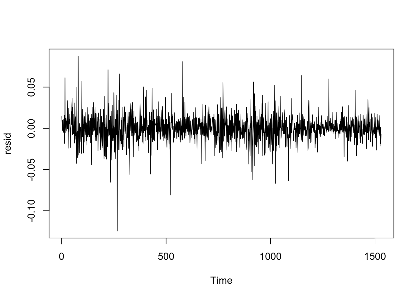
acf(resid)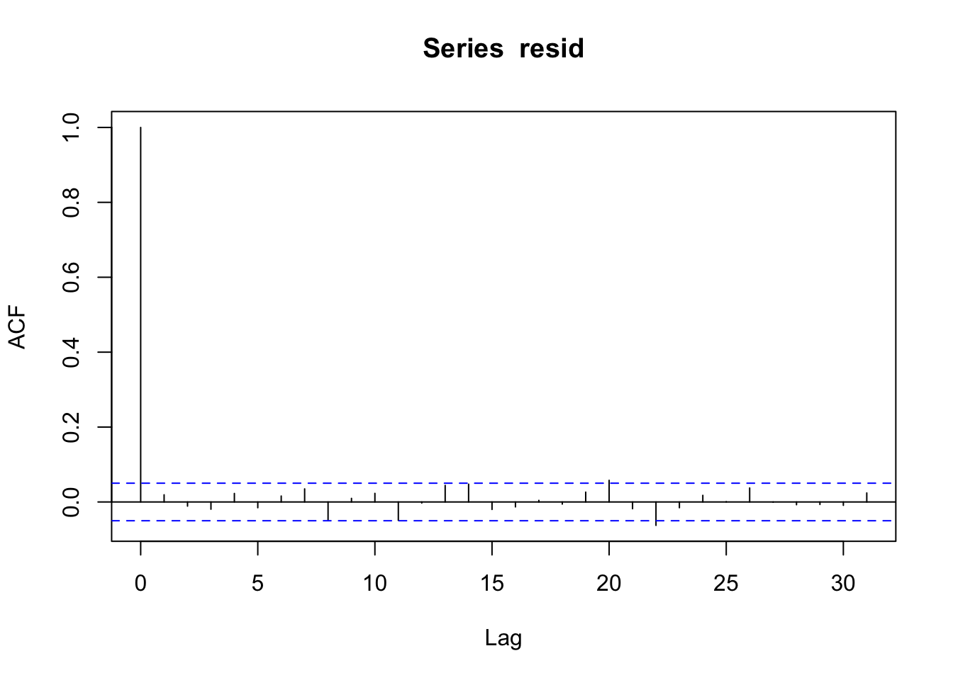
dwtest(model)##
## Durbin-Watson test
##
## data: model
## DW = 1.961, p-value = 0.2242
## alternative hypothesis: true autocorrelation is greater than 0par(mfrow = c(2, 2))
plot(model)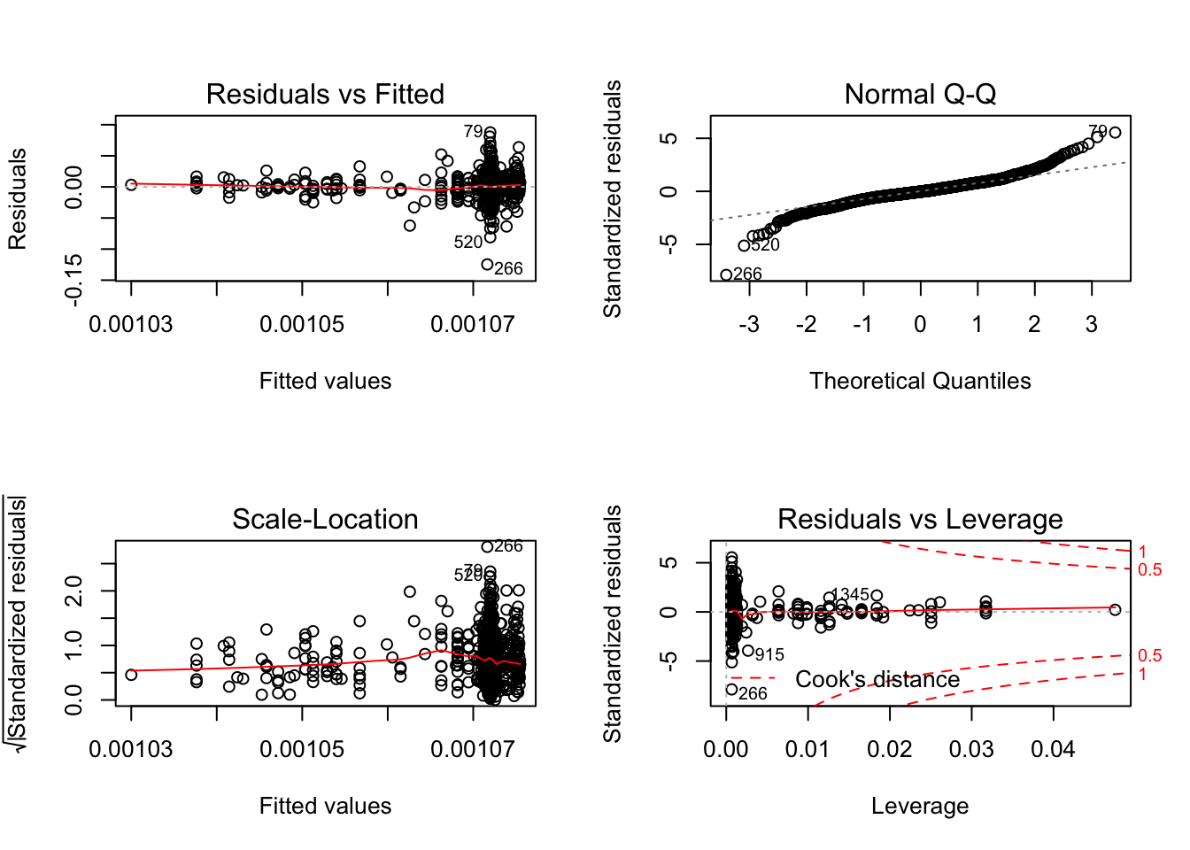
- Non-constant variance of error terms (heteroskedasticity)
- Methods to detect heterokedasticity:
- Breusch-Pagan test, White test
- Residual plot
- Methods to correct heteroskedasticity:
- Transform the response \(Y\) using a concave function such as \(\text{log}Y\) or \(\sqrt{Y}\). Such a transformation results in a greater amount of shrinkage of the larger responses, leading to a reduction in heteroscedasticity.
- If the form of the heteroskedasticity is known, we can use WLS to assign less weight to observations with a higher error variance.
- For example, the \(i\)th response could be an average of \(n_i\) raw observations. If each of these raw observations is uncorrelated with variance \(\sigma^2\), then their average has variance \(\sigma_i^2 = \frac{\sigma^2}{n_i}\). In this case a simple remedy is to fit our model using weights proportional to the inverse variances, i.e., \(w_i = n_i\) in this case.
- Methods to detect heterokedasticity:
- Outliers (in the y-direction)
- A point for which \(y_i\) is far from the value predicted by the mode.
- Residual plots can be used to identify outliers, but instead of using residuals themselves, we can plot the studentized residuals, computed by dividing each residual by its estimated standard error. Observations whose studentized residuals are greater than 3 in absolute value are possible outliers.
- Linear regression is prone to chasing observations that are away from the overall trend of the majority of the data. To cure this problem, alternative metrics to SSE can be used:
- minimizing the sum of the absolute errors
- Huber function (using the squared residuals when they are small and the absolute ones when they are above a threshold)
- High leverage points (in the x-direction)
- Methods to detect high leverage points:
- Leverage statistic
- The \(i\)th diagonal element of the hat matrix \(\mathbf{X}\left(\mathbf{X}^T\mathbf{X}\right)^{-1}\mathbf{X}^T\): \[h_i = \frac{1}{n} + \frac{(x_i - \bar{x})^2}{\sum(x_i - \bar{x})^2}\]
- The leverage statistic \(h_i\) is always between \(\frac{1}{n}\) and 1, and the average leverage for all the observations is always equal to \(\frac{p + 1}{n}\). Hence, if a given observation has a leverage statistic that greatly exceeds \(\frac{p + 1}{n}\), then we may suspect that the corresponding point has high leverage.
- Cook’s distance
- Combines both leverage and outliers: \[C_i = \frac{1}{p}r_{studentized}^2\frac{h_i}{1 - h_i}\]
- Leverage statistic
- Methods to detect high leverage points:
- Collinearity
- Collinearity reduces the accuracy of the estimates of the regression coefficients, and, hence, causes the standard error for \(\beta_j\) to grow.
- Method to detect collinearity: VIF
- Method to correct collinearity: orthoganization, PCA, heuristic approach
Paritial least squares
- PCR: pre-processing predictors via PCA prior to performing regression (unsupervised)
- PLS: while the PCA linear combinations are chosen to maximally summarize predictor space variability, the PLS linear combinations of predictors are chosen to maximally summarize covariance with the response (supervised). This means that PLS finds components that maximally summarize the variation of the predictors while simultaneously requiring these components to have max correlation with the response.
Penalized models to prevent overfitting
- Ridge regression: \[SSE_{L2} = \sum_{i=1}^{n}(y_i - \hat{y_i})^2 + \lambda\sum_{j=1}^{P}\beta^2\]
- Lasso regression: \[SSE_{L1} = \sum_{i=1}^{n}(y_i - \hat{y_i})^2 + \lambda\sum_{j=1}^{P}|\beta|\]
- Ridge regression is known to shrink the coefficients of correlated predictors towards each other, allowing them to borrow strength from each other. in the extreme case of k identical predictors, they each get identical coefficients with \(\frac{1}{k}\)th the size that any single one would get if fit alone.
- Lasso, on the other hand, is somewhat indifferent to very correlated predictors, and will tend to pick one and ignore the rest (i.e., feature selection).
- Elastic net: \[SSE_{Enet} = \sum_{i=1}^{n}(y_i - \hat{y_i})^2 + \lambda_1\sum_{j=1}^{P}\beta^2 + \lambda_2\sum_{j=1}^{P}|\beta|\]
- Predictor data need to be centered and scaled first before applying regularization.
Smoothing
Regression spline
- Idea: instead of fitting a high-degree polynomial over the entire range of \(X\), piece-wise polynomial regression involves fitting separate low-degree polynomials over different regions of \(X\).
- Cubic spline:
- If we place \(K\) different knots throughout the range of \(X\), then we will end up fitting \(K + 1\) different cubic polynomials.
- The regression spline is most flexible in regions that contain a lot of knots.
- 3 additional constraints are added for cubic spline: at each knot, the fitted curve must be continuous, and so must its first and second derivatives (i.e., smooth). Hence, a cubic spline with \(K\) knots uses a total of \(K + 4\) degrees of freedom.
- Each constraint that we impose on the piecewise cubic polynomials effectively frees up one degree of freedom, by reducing the complexity of the resulting piecewise polynomial fit. \[y_i = \beta_0 + \beta_1b_1(x_i) + \beta_2b_2(x_i) +...+ \beta_{K+3}b_{K+3}(x_i) + \epsilon_i\] where \(b_i\) is the basis function. Typically, \[y_i = \beta_0 + x + x^2 + x^3 + h(x, \xi_1) + h(x, \xi_2) +...+ h(x, \xi_K)\] where \[h(x, \xi) = (x - \xi)_+^3\]
- Natural spline:
- Additional boundary constraints: the function is required to be linear at the boundary (in the region where X is smaller than the smallest knot, or larger than the largest knot).
Smoothing spline
- Minimize \[\sum_{i=1}^n(y_i - g(x_i))^2 + \lambda\int g''(t)^2dt\] where \(\lambda\) is a nonnegative tuning parameter and \(\lambda\int g''(t)^2dt\) penalizes the variability in \(g\).
- The function \(g(x)\) that minimizes it is a natural cubic spline with knots at \(x_1, ..., x_n\).
- As \(\lambda\) increases from 0 to \(\infty\), the effective degrees of freedom decrease from \(n\) to 2.
Local regression
- Computes the fit at a target point \(x_0\) using only the nearby training observations.
- Needs to determine the span, \(s = \frac{k}{n}\), which is the fraction of training points whose \(x_i\) are closest to \(x_0\). The smaller the value of \(s\), the more local and wiggly will be our fit; alternatively, a very large value of \(s\) will lead to a global fit to the data using all of the training observations.
Generalized additive models
- A general framework for extending a standard linear model by allowing non-linear functions of each of the variables, while maintaining additivity. \[y_i = \beta_0 + f_1(x_{i1}) + f_2(x_{i2}) + \dots + f_p(x_{ip}) + \epsilon_i\] where \(f_j(x_{ij})\) is the non-linear functions.
- GAMs provide a useful compromise between linear and fully nonparametric models.
GAMs for logistic regression
\[log\Big(\frac{p}{1 - p}\Big) = \beta_0 + f_1(x_1) + \dots + f_p(x_P)\]
Multivariate adaptive regression splines (MARS)
- MARS creates a piecewise linear model where each new surrogate feature models an isolated portion of the original data.
- Each data points for each predictor is evaluated as a candidate cut point by creating a linear regression model with the candidate features, and the corresponding model error is calculated. The predictor/cut point combination that achieves the smallest error is used (as \(h(x - a)\) and \(h(a - x)\)).
- After the initial model is created with the first 2 features, the model conducts another exhaustive search to find the next set of features that, given the initial set, yield the best model fit.
- Pruning: once the full set of features has been created, the algorithm sequentially removes individual features that do not contribute significantly to the model equation (in terms of decreases in error rate) using generalized cross-validation.
- Another pruning parameter is for the degree of the features that are added to the model (i.e., interaction terms).
- Extension to classification: FDA
Neural networks
- Hidden units: \[h_k(X) = g\Big(\beta_{0k} + \sum_{i=1}^{P}x_j\beta_{jk}\Big)\] where \[g(u) = \frac{1}{1 + e^{-u}}\] and \(k\) is the number of hidden units in a layer
- Combining hidden units (single-layer): \[f(x) = \gamma_0 + \sum_{k=1}^{H}\gamma_kh_k\]
- The back-propagation algorithm uses derivatives to find the optimal parameters. However, it is common that a solution is not a global solution.
- Regularization using weight decay (single-layer): \[\sum_{i=1}^{n}(y_i - f_i(x))^2 + \lambda\sum_{k=1}^{H}\sum_{j=0}^{P}\beta_{jk}^2 + \lambda\sum_{k=0}^{H}\gamma_k^2\]
For classification
- The softmax transformation is used to ensure the outputs of the neural network lie between 0 and 1: \[f_{il}^*(x) = \frac{e^{f_{il}(x)}}{\sum_le^{f_{il}(x)}}\] where \(f_{il}(x)\) is the model prediction of the \(l\)th class and the \(i\)th sample.
- Optimization criteria:
- minimize sum of squares of errors: \[\sum_{l=1}^C\sum_{i=1}^n(y_{il} - f_{il}^*(x))^2\]
- maximize entropy: \[\sum_{l=1}^C\sum_{i=1}^ny_{il}\text{ln}f_{il}^*(x)\] although studies have shown that differences in performance tend to be negligible, the entropy function should more accurately estimate small probabilities than those generated by the squared-error function.
Support vector machines
Hyperplane
- In a \(p\)-dimensional space, a hyperplane is a flat affine subspace of dimension \(p - 1\). The word affine indicates that the subspace need not pass through the origin. \[\beta_0 + \beta_1X_1 + \beta_2X_2 + \dots + \beta_pX_p = 0\]
- The maximal margin hyperplane is the separating hyperplane for which the margin is largest—that is, it is the hyperplane that has the farthest minimum distance to the training observations.
- The maximal margin hyperplane depends directly on the support vectors, but not on the other observations.
SVM for classificatoin
- Optimization: \[max_{\beta_0, \beta_1, \dots, \beta_p}M\] \[\text{subject to }\sum_{j=1}^p\beta_j^2 = 1\] \[y_i(\beta_0 + \beta_1x_{i1} + \beta_2x_{i2} + \dots + \beta_px_{ip}) \ge M \text{ } \forall i = 1, 2, \dots, n.\]
- The first constraint ensure that the perpendicular distance from the \(i\)th observation to the hyperplane is given by \[y_i(\beta_0 + \beta_1x_{i1} + \beta_2x_{i2} + \dots + \beta_px_{ip})\]
- The 2 constraints ensure that each observation is on the correct side of the hyperplane and at least a distance M from the hyperplane.
- Sometimes a a separating hyperplane doesn’t exist; even if it does, it may lead to sensitivity to individual observations. Hence, an alternative classifier that allows misclassification solves the following optimization problem: \[max_{\beta_0, \beta_1, \dots, \beta_p, \epsilon_1, \epsilon_2, \dots, \epsilon_n}M\] \[\text{subject to }\sum_{j=1}^p\beta_j^2 = 1\] \[y_i(\beta_0 + \beta_1x_{i1} + \beta_2x_{i2} + \dots + \beta_px_{ip}) \ge M(1 - \epsilon_i)\] \[\epsilon_i \ge 0, \sum_{i=1}^n\epsilon_i \le C\]
- \(\epsilon_1, \epsilon_2, \dots, \epsilon_n\) are slack variables that allow individual observations to be on the wrong side of the margin or the hyperplane.
- If \(\epsilon_i > 0\) then the \(i\)th observation is on the wrong side of the margin.
- If \(\epsilon_i > 1\) then it is on the wrong side of the hyperplane.
- \(C\) is the budget for the amount that the margin can be violated by the \(n\) observations. As the budget \(C\) increases, we become more tolerant of violations to the margin, and so the margin will widen.
- Observations that lie directly on the margin, or on the wrong side of the margin for their class, are support vectors and affect the support vector classifier. Hence, SVM is quite robust to the behavior of observations that are far away from the hyperplane.
- \(\epsilon_1, \epsilon_2, \dots, \epsilon_n\) are slack variables that allow individual observations to be on the wrong side of the margin or the hyperplane.
- The classification function for a new sample can be written as \[f(\mathbf{u}) = \beta_0 + \mathbf{\beta'u} = \beta_0 + \sum_{j=1}^P\beta_ju_j = \beta_0 + \sum_{i=1}^ny_i\alpha_ix_i'\mathbf{u}\] where \(\alpha_i\) is nonzero only for the support vectors.
- The dot product, \(x_i'\mathbf{u}\), can be written as a product of the distance of \(x_i\) from the origin, the distance of \(\mathbf{u}\) from the origin, and the cosine of the angle between \(x_i\) and \(\mathbf{u}\). In other words, it measures the similarity between \(x_i\) and \(\mathbf{u}\).
- More generally, given the dot product of the new samples and the training samples, the equation can be written as: \[f(\mathbf{u}) = \beta_0 + \sum_{i=1}^ny_i\alpha_iK(\mathbf{x_i}, \mathbf{u})\] where \(K(\cdot)\) is called the kernal function, which quantifies the similarity of two observations. Other types of kernel functions can be used to encompass nonlinear functions of the predictors: \[\text{polynomial} = (\phi(\mathbf{x'u}) + 1)^{degree}\] \[\text{radial basis function} = \exp(-\sigma||\mathbf{x} - \mathbf{u}||^2)\] \[\text{hyperbolic tangent} = \tanh(\phi(\mathbf{x'u}) + 1)\] where \(\phi\) and \(\sigma\) are scaling parameters.
Relationship with logistic regression
- It can be shown that optimization criterion for SVM can be rewritten to the form of “Loss + Penalty” as follows: \[minimize_{\beta_0, \beta_1, \dots, \beta_p}{\sum_{i=1}^nmax[0, 1 - y_if(x_i)] + \lambda\sum_{j=1}^p\beta_j^2}\]
- The hinge loss function is closely related to the loss function used in logistic regression as shown below:
library(reshape2)
library(ggplot2)
yx = seq(-5, 4, .01)
l1 = log(1 + exp(-yx))
l2 = ifelse(1 - yx < 0, 0, 1 - yx)
df = data.frame(cbind(yx, l1, l2))
df = melt(df, id = 'yx')
ggplot(df, aes(x = yx, y = value, colour = variable)) + geom_line() +
scale_colour_discrete(name = 'Model', labels = c('Logistic Regression Loss', 'SVM Loss')) + xlab('yf(x)') + ylab('Loss')
- Due to the similarities between their loss functions, logistic regression and the support vector classifier often give very similar results. When the classes are well separated, SVMs tend to behave better than logistic regression; in more overlapping regimes, logistic regression is often preferred.
SVM for regression
- \(\epsilon\)-insensitive loss function:
- data points with residuals within the threshold (i.e., samples that the model fits well) do not contribute to the regression fit.
- data points with an absolute difference greater than the threshold contribute a linear-scale amount.
- As a result, the poorly-predicted points (the “outliers” in the extreme case) are the only points that define the regression line.
- The SVM regression coefficients minimize \[cost\sum_{i=1}^{n}L_\epsilon(y_i - \hat{y_i}) + \sum_{j=1}^{P}\beta_j^2\] where \(L_\epsilon(\cdot)\) is the \(\epsilon\)-insensitive function and \(cost\) is the cost penalty as the reverse of the \(\lambda\) used in regularized regressions or neural networks.
- The linear SVM predictor function for a new sample \(u\) is written as: \[\hat{y} = \beta_0 + \beta_1u_1 + \dots + \beta_Pu_P = \beta_0 + \sum_{j=1}^{P}\beta_ju_j = \beta_0 + \sum_{j=1}^{P}\sum_{i=1}^{n}\alpha_ix_{ij}u_j = \beta_0 + \sum_{i=1}^{n}\alpha_i\Big(\sum_{j=1}^{P}x_{ij}u_j\Big)\]
- Each data points are used in the prediction, however,
- For training set samples that are within \(\pm\epsilon\) of the regression line, the \(\alpha\) parameters are 0, indicating they have no impact on prediction.
- The rest of the data points with non-zero \(\alpha\) are called the support vectors.
K-nearest neighbors
- For classification, KNN estimates the conditional probability for class \(j\) as the fraction of points in \(N_0\) whose response values equal \(j\): \[Pr(Y = j|X = x_0) = \frac{1}{K}\sum_{i \in N_0}I(y_i = j)\] It then applies Bayes rule and classifies the test observation \(x_0\) to the class with the largest probability.
- For regression, KNN estimates \(f(x_0)\) using the average of all the training responses in \(N_0\): \[\hat{f(x_0)} = \frac{1}{K}\sum_{i \in N_0}y_i\]
- Predictor data need to be centered and scaled prior to performing KNN.
- Also need to remove irrelevant or noisy predictors.
- Suffers from curse of dimensionality: the \(K\) observations that are nearest to a given test observation \(x_0\) may be very far away from \(x_0\) in \(p\)-dimensional space when \(p\) is large.
Trees
Regression trees
- SSE is used to find the optimal split.
- Each terminal node uses the average of the training set outcomes in that node for prediction.
- The top-down approach (aka, recursive binary splitting) is greedy because at each step of the tree-building process, the best split is made at that particular step, rather than looking ahead and picking a split that will lead to a better tree in some future step.
- We consider all predictors \(X_1, \dots, X_p\), and all possible values of the cutpoint for each of the predictors, and then choose the predictor and cutpoint such that the resulting tree has the lowest SSE.
- Pruning to prevent overfitting: apply cost complexity pruning to the large tree in order to obtain a sequence of best subtrees, as a function of \(C_p\). \[SSE_{C_p} = SSE + C_p \times (\text{number of terminal nodes})\]
- Handling missing data:
- When building the tree, missing data are ignored.
- For each split, a variety of alternatives, surrogate splits, are evaluated. A surrogate split is one whose results are similar to the original split actually used in the tree.
- If a surrogate split approximates the original split well, it can be used when the predictor data associated with the original split are not available.
- Variable importance: overall reduction in the optimization criteria for each predictor.
- Limitations:
- By construction, tree models partition the data into rectangular regions of the predictor space, which may result in sub-optimal predictive performance.
- An individual tree tends to be unstable. If the data are slightly altered, a completely different set of splits might be found. Ensemble methods, on the other hand, exploit this characteristic to create models that tend to have extremely good performance.
- Trees suffer from selection bias: predictors with a higher number of distinct values (including continuous variables) are favored over more granular predictors. Also, as the number of missing values increases, the selection of predictors becomes more biased.
- Correlations between predictors can dilute the importance of key predictors.
- Conditional inference trees: for a candidate split, statistical hypothesis test is used to evaluate the difference between the means of the 2 groups created by the split and a p-value is computed.
Regression model trees
- Splitting criterion: \[\text{reduction} = SD(S) - \sum_{i=1}^{P}\frac{n_i}{n} \times SD(S_i)\] where SD is the standard deviation of the dataset (\(S\) denotes the entire set and \(S_i\) denotes the \(i\)th subset) and \(n_i\) is the number of samples in partition \(i\). Hence, it determines if the total variation in the splits, weighted by sample size, is lower than in the presplit data. In subsequent split, the error associated with each linear model is used in place of \(SD(S)\).
- For a given linear model, an adjusted error rate is computed as follows: \[\text{adjusted error rate} = \frac{n^* + p}{n^* - p}\sum_{i=1}^{n^*}|y_i - \hat{y_i}|\] where \(n^*\) is the number of training set data points used to build the model and \(p\) is the number of parameters.
- Once the complete set of models have been created, each undergoes a simplification procedure to potentially drop some of the terms. Terms are dropped as long as the adjusted error rate decreases.
- Smoothing: when predicting, the new sample goes down the appropriate path, and moving from the bottom up, the linear models along that path are combined. Each time 2 predictors are combined using \[\hat{y} = \frac{n_k\hat{y_k} + c\hat{y_p}}{n_k + c}\] where \(y_k\) and \(y_p\) are the predictions from the child and parent nodes, respectively, \(n_k\) is the number of training set points in the child node, and \(c\) is a constant with a default value of 15.
- Pruning is done using the adjusted error rate.
Classification trees
- For a classification tree, we predict that each observation belongs to the most commonly occurring class of training observations in the region to which it belongs.
- Splitting criteria:
- Classification error rate: the fraction of the training observations in that region that do not belong to the most common class. \[E = 1 - max_k(\hat{p_{mk}})\] where \(\hat{p_{mk}}\) represents the proportion of training observations in the \(m\)th region that are from the \(k\)th class. However, it turns out that classification error is not sufficiently sensitive for tree-growing, and in practice two other measures are preferable.
- Gini index: \[G = \sum_{k=1}^K\hat{p_{mk}}(1 - \hat{p_{mk}})\] Gini index is a measure of node purity as a small value indicates that a node contains predominantly observations from a single class.
- Cross-entropy: \[D = -\sum_{k=1}^K\hat{p_{mk}}\text{log}\hat{p_{mk}}\] Like the Gini index, the cross-entropy will take on a small value if the \(m\)th node is pure. In fact, it turns out that the Gini index and the cross-entropy are quite similar numerically.
Rule-based models
- A rule is defined as a distinct path through a tree. One approach to creating rules from model trees is
- An initial model tree is created.
- Only the rule with the largest coverage is saved form this model. The samples covered by the rule are removed from the training set and another model tree is created with the remaining data.
- Repeat until all the training data have been covered by at least 1 rule.
Random forests
- Tree correlation prevents bagging from optimally reducing variance of the predicted values.
- Random forests randomly selects predictors (e.g., \(\sqrt{p}\)) at each split, hence reducing tree correlation.
- To produce stable results, in practice at least 1,000 trees are needed.
- Because each learner is selected independently of all previous learners, random forests is robust to a noisy response.
- Out-of-bag error rate can be used to assess the predictive performance.
- Variable importance is determined by aggregating the individual improvement values for each predictor across the forest.
Gradient boosting trees
- Boosting differs from bagging in that the trees are grown sequentially: each tree is grown using information from previously grown trees. Hence, boosting does not involve bootstrap sampling; instead each tree is fit on a modified version of the original data set.
- Tuning parameters: tree depth (or interaction depth), number of iterations, and learning rate \(\lambda\).
- Tree depth, or the number of splits, controls the complexity of the boosted ensemble (often \(d = 1\) works well, in which case each tree is a stump, consisting of a single split). This highlights one difference between boosting and random forests: in boosting, because the growth of a particular tree takes into account the other trees that have already been grown, smaller trees are typically sufficient. Using smaller trees can aid in interpretability as well; for instance, using stumps leads to an additive model.
- Unlike bagging and random forests, boosting can overfit if the number of trees/iterations is too large.
- Updating the predicted value of each sample by adding the value predicted in the current iteration to that of the previous iteration. To prevent overfitting, only a fraction of the current predicted value, as determined by \(\lambda\) is added. In general, statistical learning approaches that learn slowly tend to perform well.
- Using the residuals as the response to fit a tree. By fitting small trees to the residuals, we slowly improve \(\hat{f}\) in areas where it does not perform well. \[\hat{f(x)} \leftarrow \hat{f(x)} + \lambda\hat{f^b(x)}\] \[r_i \leftarrow r_i - \lambda\hat{f^b(x)}\] \[\hat{f(x)} = \sum_{b=1}^B\lambda\hat{f^b(x)}\]
- Stochastic gradient boosting: randomly select a fraction of the training data before constructing gradient boost trees.
Cubist
- Cubist is a rule-based model.
- Smoothing is done as follows: \[\hat{y} = a \times \hat{y_k} + (1 - a) \times \hat{y_p}\] where \[a = \frac{var(e_p) - cov(e_k, e_p)}{var(e_p - e_k)}\] where \(e_k\) and \(e_p\) are the residuals of the child and parent models, respectively. In the end, the model with the smallest RMSE has a higher weight in the smoothed model.
- Boosting(committee model): similar to GBM, the \(m\)th committee model uses an adjusted response calculated as: \[y_m^* = y - (\hat{y_{m-1}} - y)\] Hence, if a data point is underpredicted, the sample value is increased in the hope that the model will produce a larger prediction in the next iteration, and vice versa.
- Finally, when predicting a new model, the \(K\) most similar neighbors are determined from the training set and their observed outcome and predicted values are used to adjust the prediction as: \[\frac{1}{K}\sum_{l=1}^{K}w_l[t_l + (\hat{y} - \hat{t_l})]\] where \(t_l\) and \(\hat{t_l}\) are the observed and prediction for a training set neighbor, and \(w_l\) is a weight calculated using the distance of the neighbor to the new sample.
- Tuning parameters: number of committees and neighbors.
Measuring performace in classification models
- Overall accuracy
- Kappa statistic: \[Kappa = \frac{O - E}{1 - E}\] where \(O\) is the observed accuracy and \(E\) is the expected accuracy based on the marginal totals of the confusion matrix.
- Sensitivity: true positive rate
- Specificity: true negative rate = 1 - false positive rate
Linear classificatoin models
Logistic regression
- Binomial likelihood: \[L(p) = C_n^r p^r (1 - p)^{n-r}\] where \(n\) is total number of trials and \(r\) is the number of successes.
- Log odds of the event as a linear function: \[log\Big(\frac{p}{1 - p}\Big) = \beta_0 + \beta_1x_1 + \dots + \beta_Px_P\]
- Event probability: \[p = \frac{1}{1 + exp[-(\beta_0 + \beta_1x_1 + \dots + \beta_Px_P)]}\]
- Using maximum likelihood to fit a logistic regression model (given the data and given our choice of model, what value of the parameters of that model make the observed data most likely?): \[L(\beta) = \prod_{i=1}^nPr(Y = y_i|X = x_i) = \prod_{i=1}^np_i^{y_i}(1 - p_i)^{1-y_i}\] \[l(\beta) = \sum_{i=1}^n[y_i\text{log}p(x_i) + (1 - y_i)\text{log}(1 - p(x_i))]\]
Linear discriminate analysis
Given Bayes’ rule, \[Pr[Y = C_l|X] = \frac{Pr[Y = C_l] \cdot Pr[X|Y = C_l]}{Pr[X]} = \frac{Pr[Y = C_l] \cdot Pr[X|Y = C_l]}{\sum_{l=1}^{C}Pr[Y = C_l] \cdot Pr[X|Y = C_l]}\] \(X\) is classified into group \(C_l\) if \(Pr[Y = C_l] \cdot Pr[X|Y = C_l]\) has the largest value of all C classes.
Assuming the distribution of the predictors is multivariate normal with a multidimensional mean vector \(\mathbf{\mu}_l\) and covariance matrix \(\Sigma_l\), \[\text{log}(Pr[X|Y = C_l]) = \text{log} f_l(x) = \text{log} \Big(\frac{1}{(2\pi)^\frac{p}{2}|\Sigma_l|^\frac{1}{2}}exp(-\frac{1}{2}(x - \mu_l)^T\Sigma_l^{-1}(x - \mu_l)) \Big)\]
Further assuming the covariance matrices are identical across groups, the above equation is equivalent to \[x^T\Sigma^{-1}\mu_l - \frac{1}{2}\mu_l^T\Sigma^{-1}\mu_l\] Adding the prior probability, we have \[x^T\Sigma^{-1}\mu_l - \frac{1}{2}\mu_l^T\Sigma^{-1}\mu_l + \text{log}(Pr[Y = C_l])\] Without the assumption of constant covariance, the equation is no longer linear in \(X\) and is hence QDA.
LDA advantages over logistic regression:
- When the classes are well-separated, the parameter estimates for the logistic regression model are surprisingly unstable. Linear discriminant analysis does not suffer from this problem.
- If \(n\) is small and the distribution of the predictors \(X\) is approximately normal in each of the classes, the linear discriminant model is again more stable than the logistic regression model.
- Linear discriminant analysis is popular when we have more than two response classes.
LDA limitations:
- The LDA solution depends on inverting a covariance matrix - a unique solution exists only when the data contain more samples than predictors and the predictors are independent (just like in regression).
- Assumption of normal distribution and equal covariance.
Extensions to LDA:
- QDA
- RDA: \[\tilde{\Sigma_l}(\lambda) = \lambda\Sigma_l + (1 - \lambda)\Sigma\] where \(\Sigma_l\) is the covariance matrix of the \(l\)th class and \(\Sigma\) is the pooled covariance matrix across all classes.
- MDA: allows each class to be represented by multiple multivariate normal distribution. These distributions can have different means but, like LDA, the covariance structures are assumed to be the same.
Partial least squares discriminant analysis (PLSDA)
- PLSDA seeks to find optimal group separation while being guided by between-groups covariance matrix whereas PCA seeks to reduce dimension using the total variation as directed by the overall covariance matrix of the predictors.
- However, if dimension reduction is not necessary and classification is the goal, LDA will always provide a lower misclassification rate than PLS.
Penalized models
glmnetuses ridge and lasso penalties simultaneously, like the elastic net, but structures the penalty slightly differently: \[\text{log}L(p) - \lambda\Big[(1 - \alpha)\frac{1}{2}\sum_{j=1}^{P}\beta_j^2 + \alpha\sum_{j=1}^{P}|\beta_j|\Big]\] where \(\text{log}L(p)\) is the binomial or multinomial log likelihood.
Latent Dirichlet allocation
- The intuition behind LDA is that documents exhibit multiple topics.
- Document generative process:
- Randomly choose a distribution over topics. A topic is defined to be a distribution over a fixed vocabulary and is assumed to be specified before any data has been generated.
- For each document in the collection, we generate the words in a two-stage process:
- Randomly choose a distribution over topics (i.e., topic profortion).
- For each word in the document
- Randomly choose a topic from the distribution over topics in step #1.
- Randomly choose a word from the corresponding distribution over the vocabulary.
- This generative process defines a joint probability distribution over both the observed and hidden random variables. We perform data analysis by using that joint distribution to compute the conditional distribution of the hidden variables given the observed variables. This conditional distribution is also called the posterior distribution.
- The observed variables are the words of the documents
- The hidden variables are the topic structure (including the topics, per-document topic distributions, and the per-document per-word topic assignments), and the generative process is as described above. \[p(\beta_{1:K}, \theta_{1:D}, z_{1:D}|w_{1:D}) = \frac{p(\beta_{1:K}, \theta_{1:D}, z_{1:D}, w_{1:D})}{p(w_{1:D})}\]
- \(p(w_{1:D})\) is the probability of seeing the observed corpus under any topic model and, in theory, can be computed by summing the joint distribution over every possible instantiation of the hidden topic structure. Hence, it is intractable to compute.
- Topic modeling algorithms form an approximation by forming an alternative distribution over the latent topic structure that is adapted to be close to the true posterior.
- Sampling based algorithms (e.g., Gibbs sampling) attempt to collect samples from the posterior to approximate it with an empirical distribution.
- Go through each document \(d\), and randomly assign each word in the document to one of the \(K\) topics.
- To improve, go through the corpus again, and
- for each document \(d\), calculate \(p(topic_k|document_d)\), the proportion of words in document d that are currently assigned to topic \(k\), i.e., the prevelance of the topic.
- for all documents, calculate \(p(word_d|topic_k)\), the proportion of assignments to topic \(k\) over all documents that come from this word \(w\).
- Then reassign \(w\) to a new topic \(k'\) with the probability \(p(topic_{k'}|document_d) \times p(word_d|topic_{k'})\). In other words, in this step, we’re assuming that all topic assignments except for the current word in question are correct, and then updating the assignment of the current word using our model of how documents are generated.
- Repeat until converge.
- Variational methods, rather than approximating the posterior with samples, posit a parameterized family of distributions over the hidden structure and then find the member of that family that is closest to the posterior. Thus, the inference problem is transformed to an optimization problem.
- Sampling based algorithms (e.g., Gibbs sampling) attempt to collect samples from the posterior to approximate it with an empirical distribution.