Background
Earlier this year, I decided to learn French, something I’ve been thinking about for a long time. Foreign language learning has always been something magical to me: I had a great time learning English when I was at school (my mother tongue is Mandarin Chinese), so much that I would devote all my time to it and ignore my other subjects (not recommended). Hence, when I signed up for a beginner’s class in my local Alliance Française and started taking classes regularly, it felt homecoming to me. However, once I was hooked, meeting once a week quickly became too little for me, so I started to look for and adopt additional means to aid my study. Among them, Duolingo is one.1
To those who are not familiar with it, Duolingo is an app that uses gamification, beautiful designs, and the spaced repetion technique to teach users foreign languages. Personally, I found it most helpful in growing my vocabulary but not so much in developing the listening and speaking skills (at least not yet; the app does have a lot of new innovations coming out, such as a chatbot, that aim to bridge the gap). That said, I do laud the app’s effort and contributions in making language learning so easily accessible and I’m excited and eager for its future innovations.
Data from Duolingo
A couple months ago, I came across this blog post and the accompanying paper written by Duolingo’s research team (Settles and Meeder 2016) on how they developed half-life regression to model the forgetting curve for each user and each word in order to decide when to show a certain word to help people remember it. Along with the blog post, the team released the data they used in the research, which contains “the 13 million Duolingo student learning traces used in [their] experiments.” In particular, each record represents a word being shown to a given user in a given learning session and includes various features for this pair such as the attributes of the word itself (e.g., language, part-of-speech tagging) and the user (e.g., the learner’s track record related to this particular word), as well as whether the user was able to correctly recall this word at the moment. For more information, you can refer to the data dictionary posted on the repo’s readme page.
As a data scientist and a language learner myself, this dataset is extremely interesting to me and reading the paper alone is not enough to sate my curiosity, so I decided to download the data and play around with it myself, which resulted in the following analysis and this blog post.
Analysis goal
The goal of my analysis is to understand and model what drives a word to be correctly recalled. The factors I considered mainly come from three categories:
- The word: including which language it comes from, what function it serves in a sentence, and how different it is from its root (e.g., went vs. go in English).
- The user: how motivated the user is (as evidenced by the number of exercises he/she has completed before the current lesson) and how good he/she is at recalling a word in general (based on his/her historical track record).
- The user and the word: these are basically features related to the forgetting curve, including when the user saw the word last time, how many times he/she has seen it, and how many times he/she was able to recall it correctly.
In the section below, I’m going to explore each of these categories in detail, but first I need to determine what my response variable is, i.e., what I should use to define if a word is recalled correctly.
In the dataset from Duolingo, there is a variable called p_recall which is computed as the % of time a given word is correctly recalled in a given session (i.e., session_correct / session_seen). However, I am not convinced that this is an accurate measure of a person’s likelihood of correctly recalling a word because the metric is contaminated by the short-term reinforcement. For example, if a person incorrectly recalls a word for the first time in the current session, Duolingo is likely to show it again at the end, and if he/she gets it right this time, the p_recall, which is calculated at the end of the lesson, would be 0.5. However, what I’m more interested in is the user’s ability to recall it before the session so that I would know whether to show it to the user or not, which has no direct relationship with this 0.5 except it should also be less than 1.
Because of that, I decided to turn p_recall into a binary variable to indicate whether the user is able to correctly recall a given word the first time it is shown in a given lesson. The dataset doesn’t have a column indicating the first response but in my experience, if a word is correctly recalled in a review session, it will not be shown again. Hence, I assume a perfect recall rate (i.e., p_recall = 1) indicates the person got it right the first time.2
# create boolean variable to indicate whether a word is recalled correctly without making any mistake
duo = duo %>%
  mutate(no_mistake = p_recall == 1)

mean(duo$no_mistake)  # 83.8%
As shown above, in the dataset, 84% of the words are correctly recalled at the first attempt - nice work!
Next, I split the dataset into training and testing sets and performed the following exploratory analysis using the training set only.
# split into training and test sets and perform all exploratory analysis on the training set only
set.seed(123456)
ix = caret::createDataPartition(duo$no_mistake, p = .7, list = F)

duo_train = duo[ix, ]
duo_test = duo[-ix, ]
Exploratory analysis
The words
First, let’s analyze the correct rate for each word and get a sense of what makes a word easy to recall. To do that, let’s start with the learning languages.
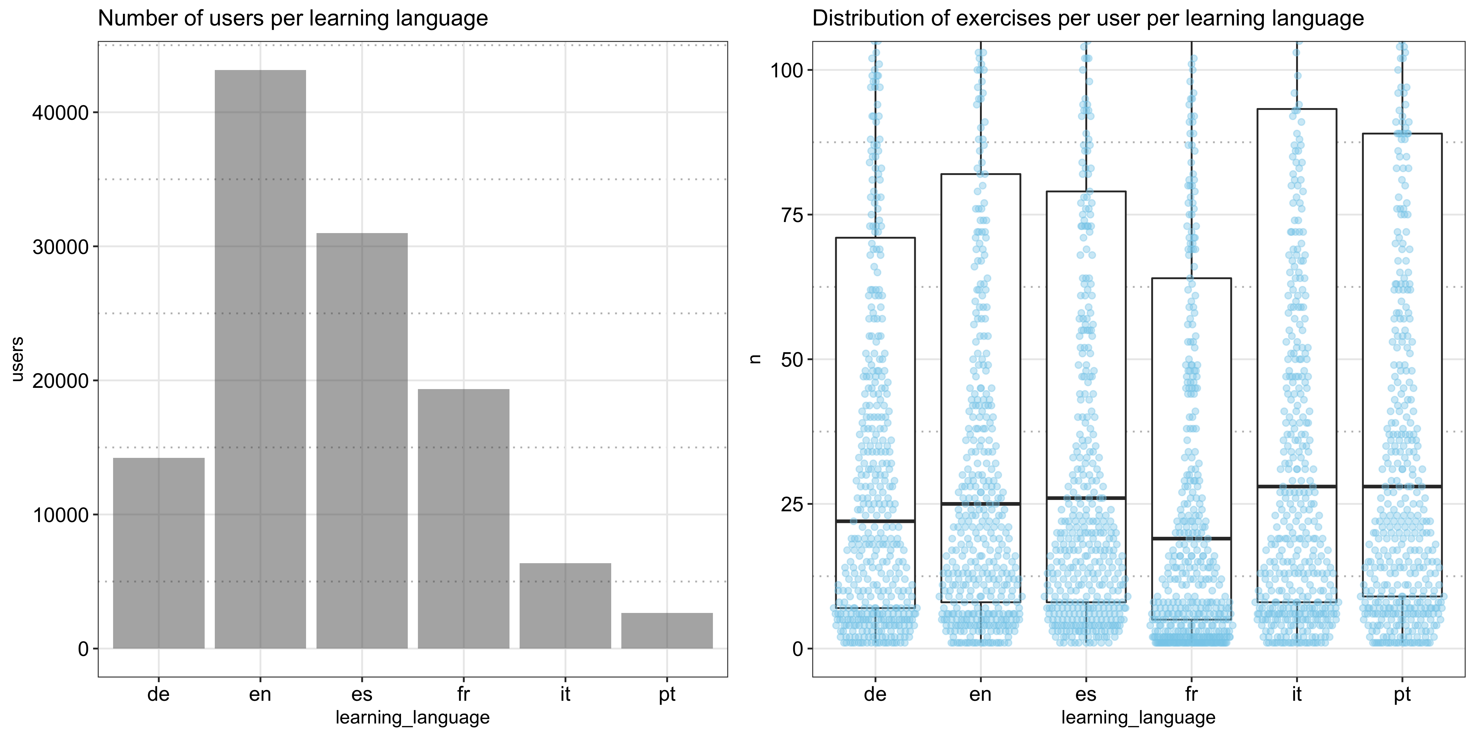
The following plot shows the number of users learning each language and the distribution of the number of exercises per user (measured by the row count, not accounting for the reinforcement of the same word in the same session). Based on the data, English is the most popular language to learn, followed by Spanish and French, and French learners seem to do fewer exercises than the others:
It’s also interesting to see what languages different language speakers study, which we can tell by creating a cross tabulation between ui_language and learning_language like below:
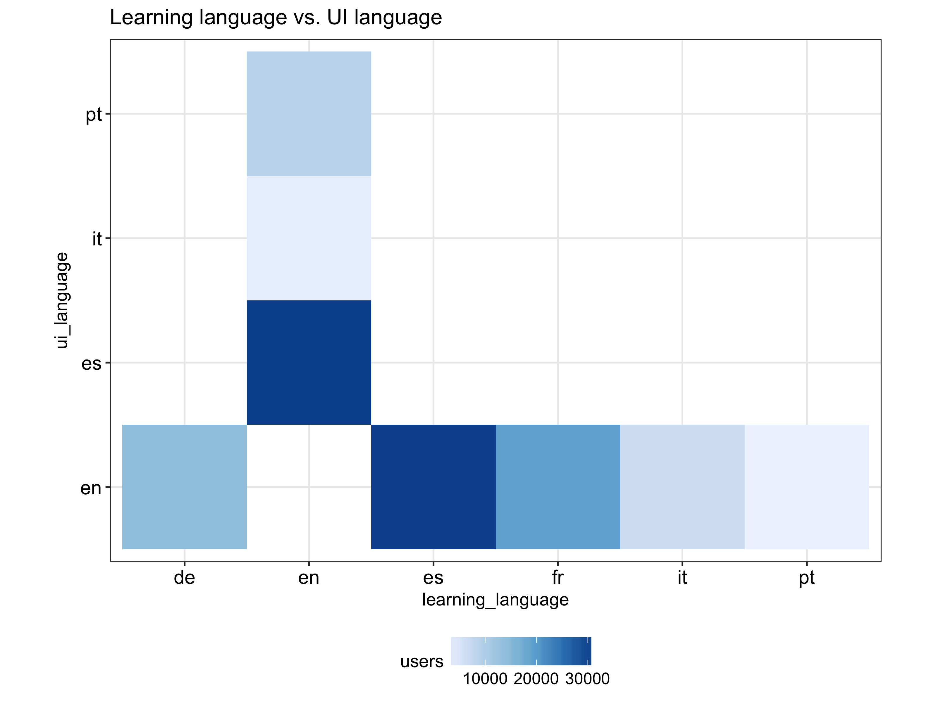
As expected, English is being learned exclusively by non-English speakers but, a bit surprisingly (at least to me), the other languages are only being learned by English speakers. However, this may not reflect the current landscape given that we don’t know how the sample was selected and that the data is dated 4 years ago.
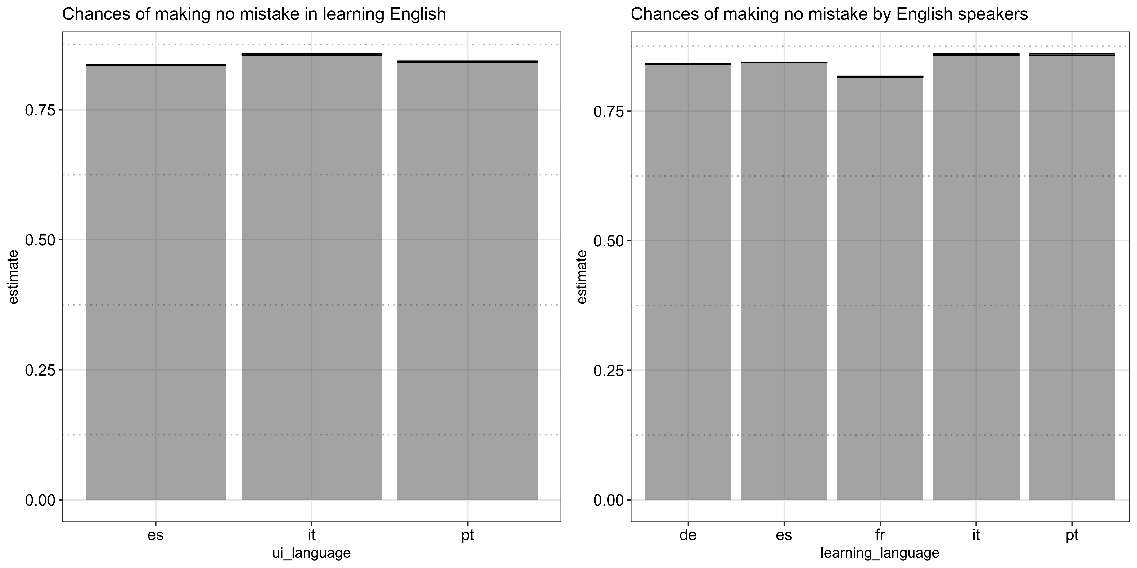
Now let’s look at the rate of successfully recalling a word per each language. As shown in the following plot, although all pretty close, Italian speakers appear to be the best in learning English and English speakers also happen to learn Italian the best, in addition to Portuguese, and struggle the most in French, which may explain the fewer number of exercises completed:
Moving on to the actual words being learned, my question for this is, aside from the language itself, what makes a word hard or easy to learn. To do that, I need to first parse out the word (surface_form), the root (lemma), and the part-of-speech tagging (pos) from the column lexeme_string:
## `lexeme_string`
### parse out `surface_form` and `lemma`
duo_train = duo_train %>%
  mutate(surface_form_lemma_pos = sub('^(.*?/.*?<.*?)>.*$', '\\1', lexeme_string),
         surface_form_lemma_pos = gsub('<([^*]*)$', ';\\1', surface_form_lemma_pos)) %>%
  separate(surface_form_lemma_pos, into = c('surface_form', 'lemma', 'pos'), sep = '/|;', remove = F) %>%
  mutate(pos = ifelse(grepl('@', pos), 'missing', pos))

### for `surface_form` wildcards, assume it is the same as `lemma`
duo_train = duo_train %>%
  mutate(surface_form = ifelse(grepl('<.+>', surface_form), lemma, surface_form))
Note in doing so, I made an assumption about the wildcard surface_form which the data dictionary describes as “refer[ing] to a ‘generic’ lexeme without any specific surface form.” Without a better understanding of what they really are, I assume they are exactly the same as their roots, lemma.
After parsing out the surface_form, for each of them, I first computed its rate of being correctly recalled:
### compute no mistake rate per word
surface_forms = duo_train %>%
  group_by(learning_language, surface_form_lemma_pos, surface_form, lemma, pos) %>%
  summarise(n = n(),
            no_mistake = sum(no_mistake)) %>%
  mutate(prc_no_mistake = no_mistake / n)
However, the problem of using the raw rate as is is that there are a lot of words that have only a few observations and, for them, I simply don’t have enough evidence to determine if the observed rate is trustworthy or not (e.g., a word that has only appeared once in the dataset can only have a rate of either 0 or 1). To deal with the issue, I used David Robinson’s handy package ebbr to fit a beta distribution to the data using only words with at least 50 observations3 and use it as the prior to compute the posterior estimate of the success rate. Because beta is the conjugate prior to the binomial distribution, the posterior estimate also follows a beta distribution with a mean of
$$\frac{\text{number of times the word is correctly recalled} + \alpha}{\text{number of times the word is shown} + \alpha + \beta}$$
Where $\alpha$ and $\beta$ are the two shape parameters estimated in the first step. This technique is called Empirical Bayes and you can read more about it in David’s awesome blog series and his accompanying book (David Robinson 2017).
Below is my implementation using ebbr:
### function to fit a beta prior to each language's rate of no mistake
fit_beta_prior = function(df, x = 'no_mistake', n = 'n') {
  # filter to subjects (e.g., words, users) with at least 50 occurrences
  # (based on EDA, this is enough to create a smooth distribution)
  df = df %>%
    mutate_('no_mistake' = x,
            'n' = n) %>%
    filter(n >= 50) %>%
    mutate(prc_no_mistake = no_mistake / n)

  return_values = list()

  # fit prior
  return_values$prior = df %>%
    ebb_fit_prior(no_mistake, n)

  # extract prior mean
  return_values$prior_mean = return_values$prior$parameters$alpha / (return_values$prior$parameters$alpha + return_values$prior$parameters$beta)

  # visualize the fit
  label = paste0(
    'alpha: ', round(return_values$prior$parameters$alpha, 2),
    '\nbeta: ', round(return_values$prior$parameters$beta, 2),
    '\nprior mean: ', round(return_values$prior_mean, 2),
    '\n'
  )

  return_values$fit_plt =
    ggplot(df) +
    geom_histogram(aes(x = prc_no_mistake, y = ..density..), alpha = .5) +
    stat_function(fun = function(x) dbeta(x, return_values$prior$parameters$alpha, return_values$prior$parameters$beta), colour = 'red', size = 1) +
    annotate(geom = 'text', x = 0, y = 0, label = label, hjust = 0, vjust = 0) +
    better_theme()

  return_values
}
Applying the above function to the data per language:
### nest by language and fit a beta prior per language
surface_forms_ns_by_lang = surface_forms %>%
  group_by(learning_language) %>%
  nest() %>%
  mutate(prior = map(data, fit_beta_prior))
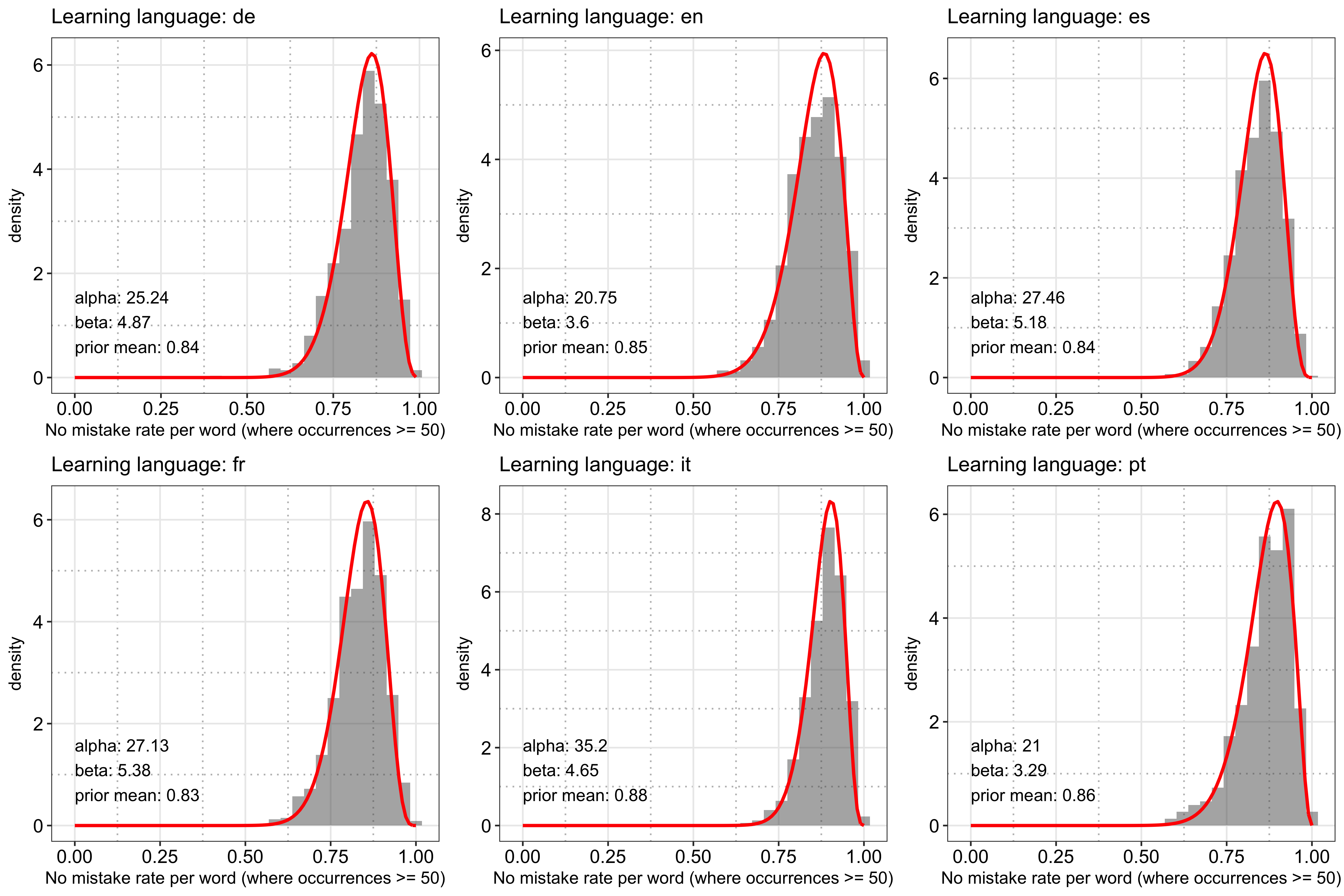
First, let’s examine how good the fit is. The following plot shows the distribution of the raw success rate per language computed in the beginning (using words with at least 50 records) and the fitted beta prior. Overall, it looks like the fit is able to capture the shape of the raw data decently:
Next, I applied the fitted prior to the whole dataset (including words with fewer than 50 records) to estimate the mean and the credible interval of the posterior success rate:
### apply the prior to the data to estimate the posterior no mistake rate
surface_forms_ns_by_lang = surface_forms_ns_by_lang %>%
  mutate(data = map2(data, prior, function(df, prior) augment(prior$prior, df)))
Using the posterior estimates, we can now get a better sense of how hard or easy a word is. To illustrate, I plotted the 10 hardest and 10 easiest words to learn per language based on the posterior mean (like the raw data, each word in the plot is represented as surface_form/lemma;pos):
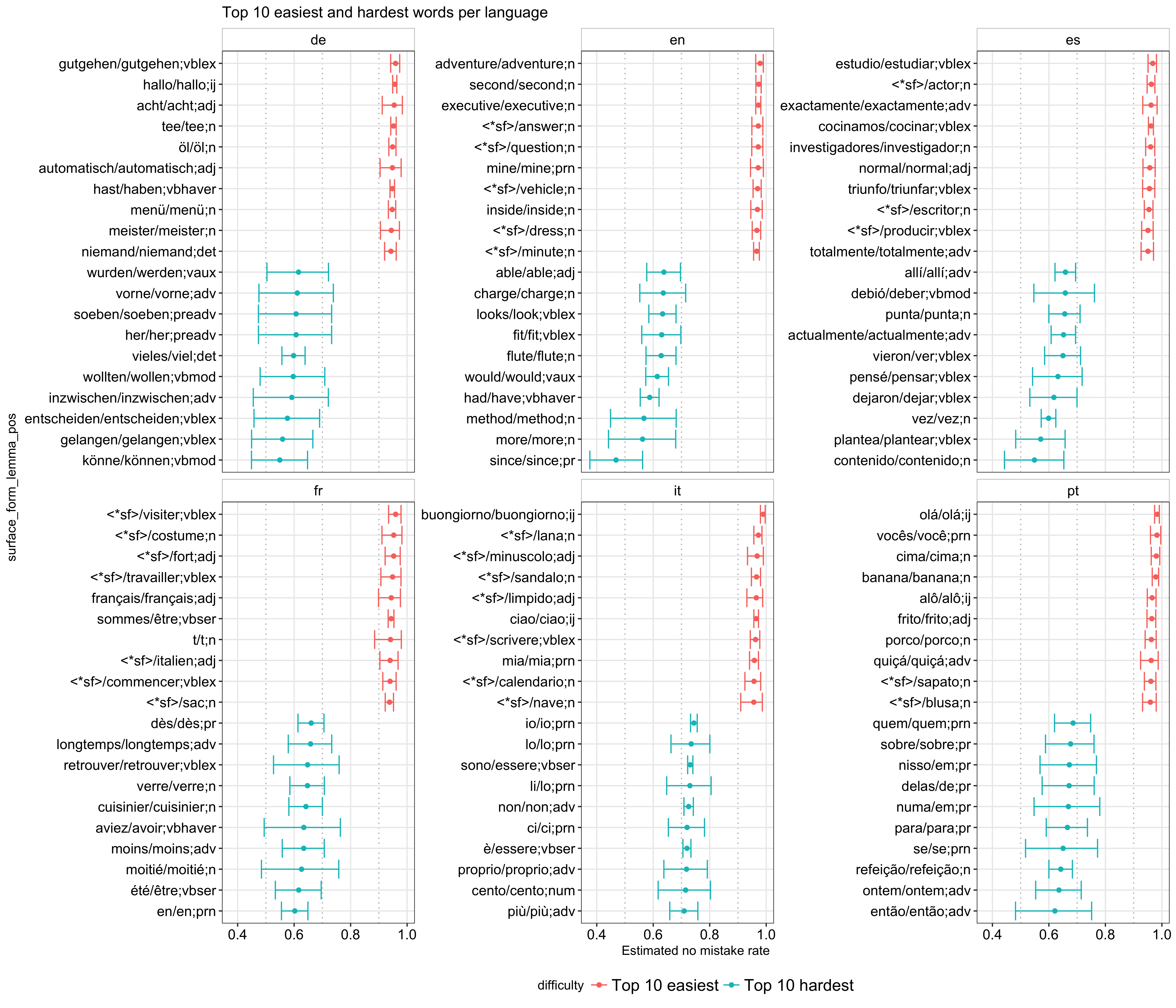
A few interesting things I noticed are:
- In general, the hardest words have a wider credible interval than the easiest ones, which indicates that they have fewer observations and, thereby, fewer people have attempted at them. If I have to guess, some of these are probably words from the more advanced part of a course and are more difficult by nature (e.g., the imperfect form aviez in French).
- Comparing
surface_formwith itslemma, I found that many of the easiest words have the same form with its root (or are wildcards, which I assume is the same case in my analysis) whereas many of the hardest ones have different forms from their root. - Related to the previous observation, there are more nouns in the easiest category while there are more verbs, propositions, and words with abstract meanings in the hardest one.
The first observation, although interesting, is not very actionable unless we know the course structure, which I don’t. Simply relying on the amount of records we have for each word is problematic because, when a new word is added, we can’t just assume it is difficult. However, if we know it is meant to be added to the later part of a course, we can reasonably assume it is one of the harder ones. By contrast, the other two observations are more useful in my analysis and are further explored below.
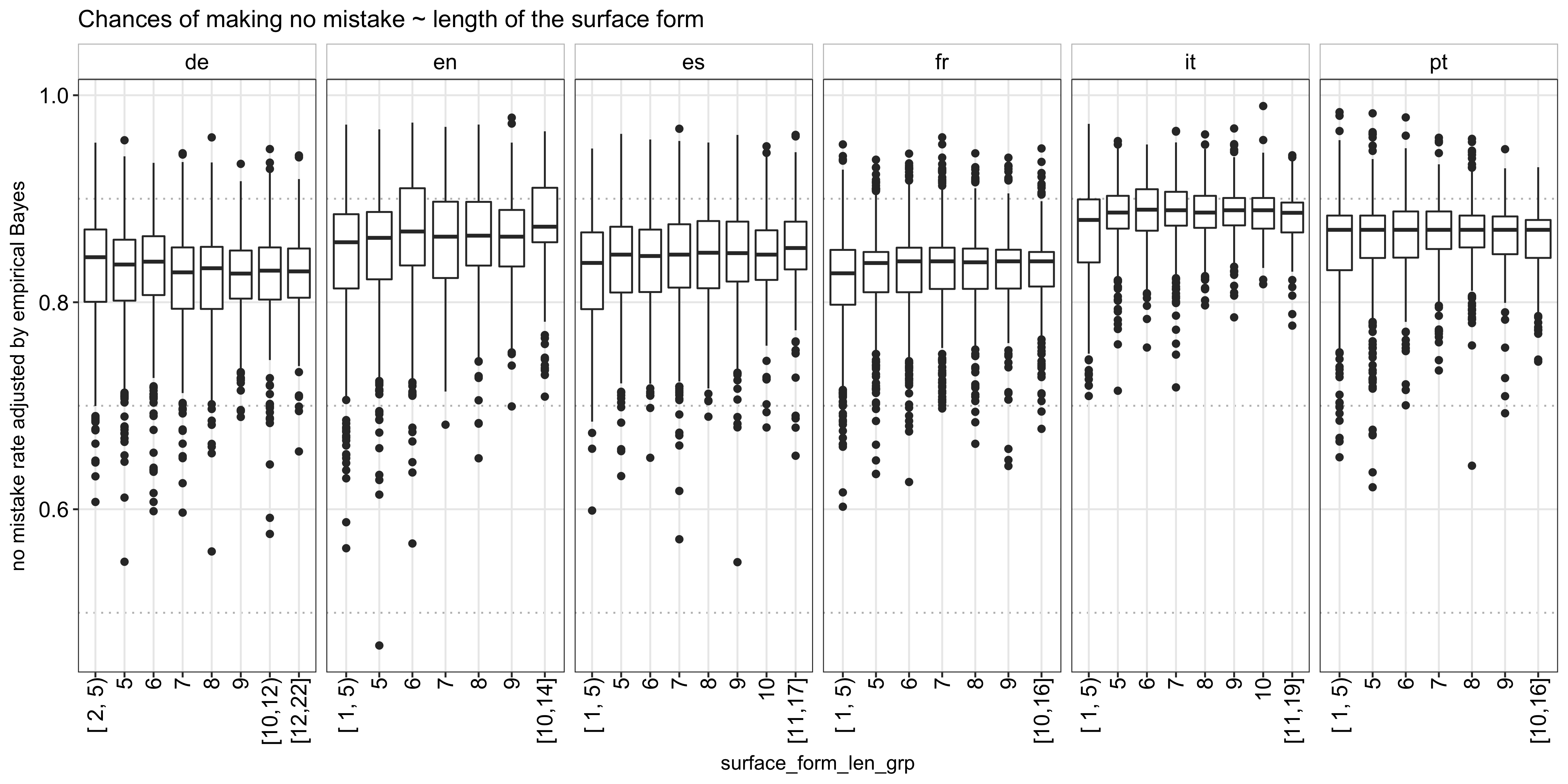
Using the mean of the posterior estimate per word, I set to explore what makes a word hard or easy to learn, which would inform my model training later on. First, I tried to see if the length of a word has anything to do with its difficulty. The following plot shows the distribution of the posterior mean per word length. It looks like, aside from English and Spanish, for which a longer word length is somewhat associated with a higher success rate, the relationship is not very clear:
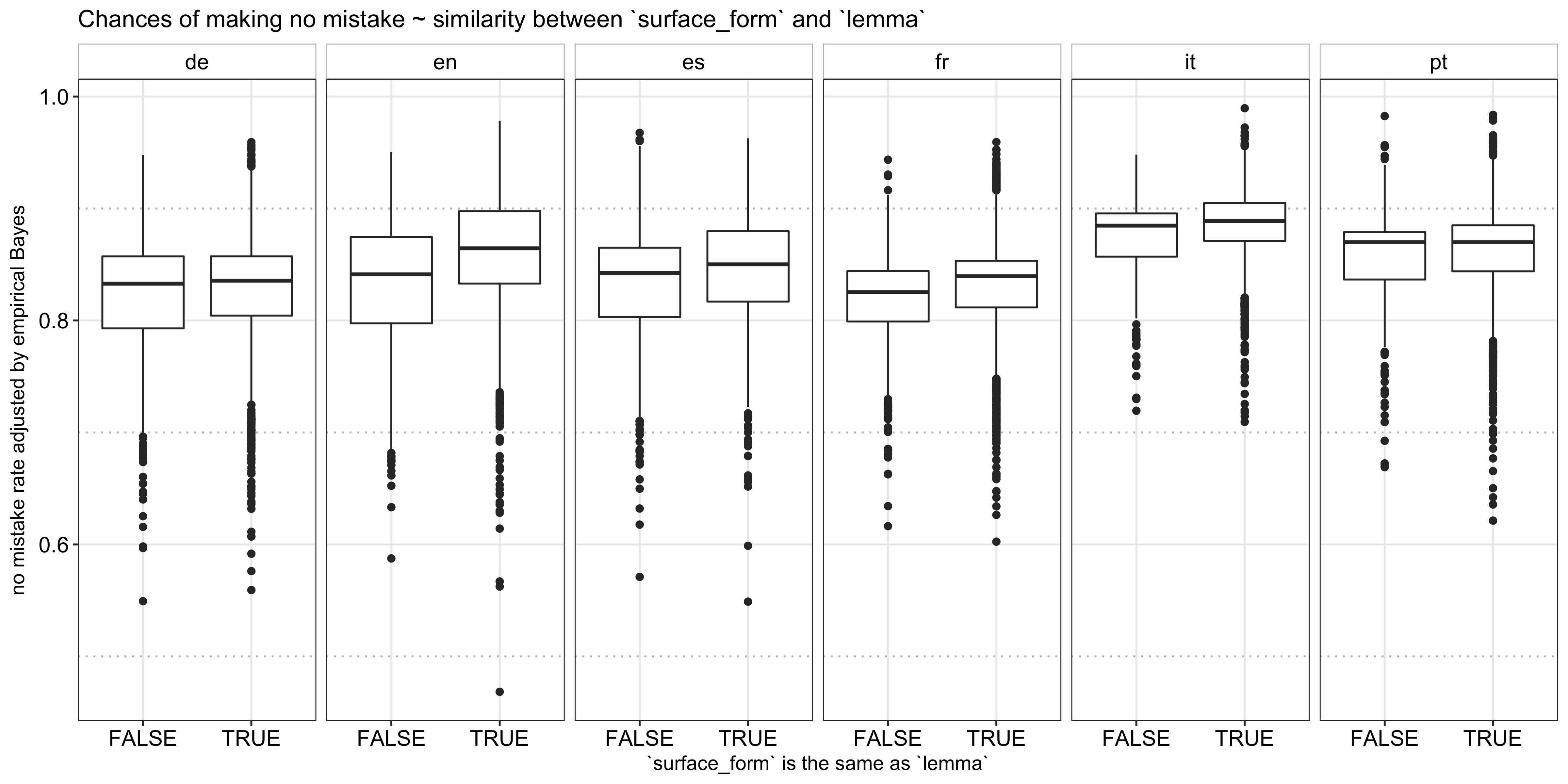
Next, I explored the second observation above and found that 74% of the words are exactly the same as their root (i.e., surface_form == lemma or are wildcards). Given the prevalence, I didn’t feel the need to compute a further fine-grained similarity metric and simply compared the success rate between words that are and are not exactly the same as their roots. As shown below, the former indeed has a higher recall rate:
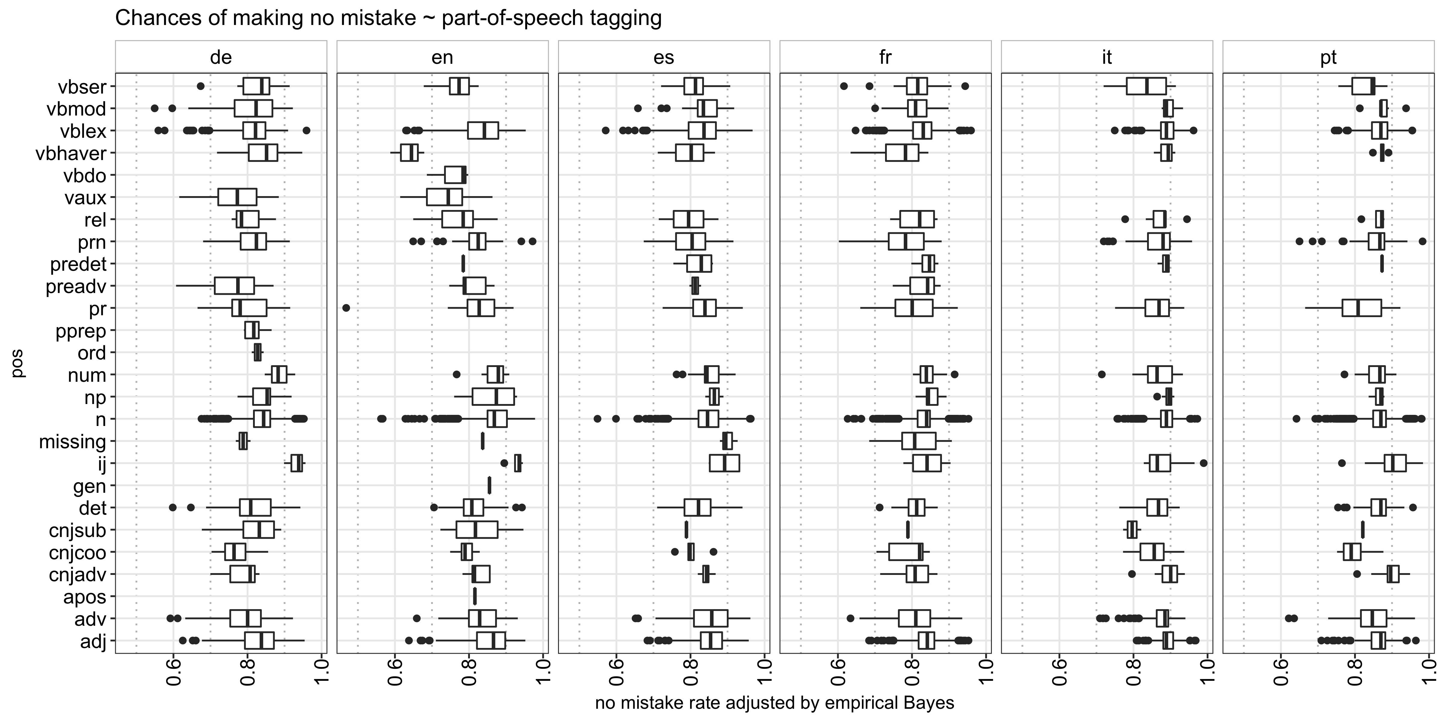
Lastly, I analyzed the impact each POS has on the success rate and found that, in general, interjections (e.g., hello and bye in English) and nouns are the easiest to learn across all languages, which makes sense because those are usually the first things we learn, whereas the different verb forms are the hardest:
Above is all the analysis I did for the words themselves. Next, let’s move on to the users.
The users
For each user, I was mainly interested in measuring how motivated he/she is in learning a language, as evidenced by the number of completed exercises, and how good he/she is in general, as reflected by his/her historical success rate across all words. As the goal is still to predict a user’s performance in the current session, I computed these metrics prior to a given session:4
### count the number of exercises a user has done and the success rate before the current session
duo_train_per_user_per_session = duo_train %>%
  group_by(learning_language, user_id, timestamp) %>%
  summarise(n = n(),
            no_mistake = sum(no_mistake)) %>%
  arrange(learning_language, user_id, timestamp) %>%
  mutate(prior_exercises_per_user = lag(cumsum(n)),
         prior_no_mistake_per_user = lag(cumsum(no_mistake)),
         prior_exercises_per_user = ifelse(is.na(prior_exercises_per_user), 0, prior_exercises_per_user),
         prior_no_mistake_per_user = ifelse(is.na(prior_no_mistake_per_user), 0, prior_no_mistake_per_user))
For the prior success rate, we run into the same problem as before in that some users do not have enough prior history for us to assess their track records reliably (for some, we don’t even have any). Hence, I used Empirical Bayes again to adjust the raw previous success rate (code omitted). For those we don’t have any prior information on, this defaults to the prior mean, which I think is a reasonable assumption.
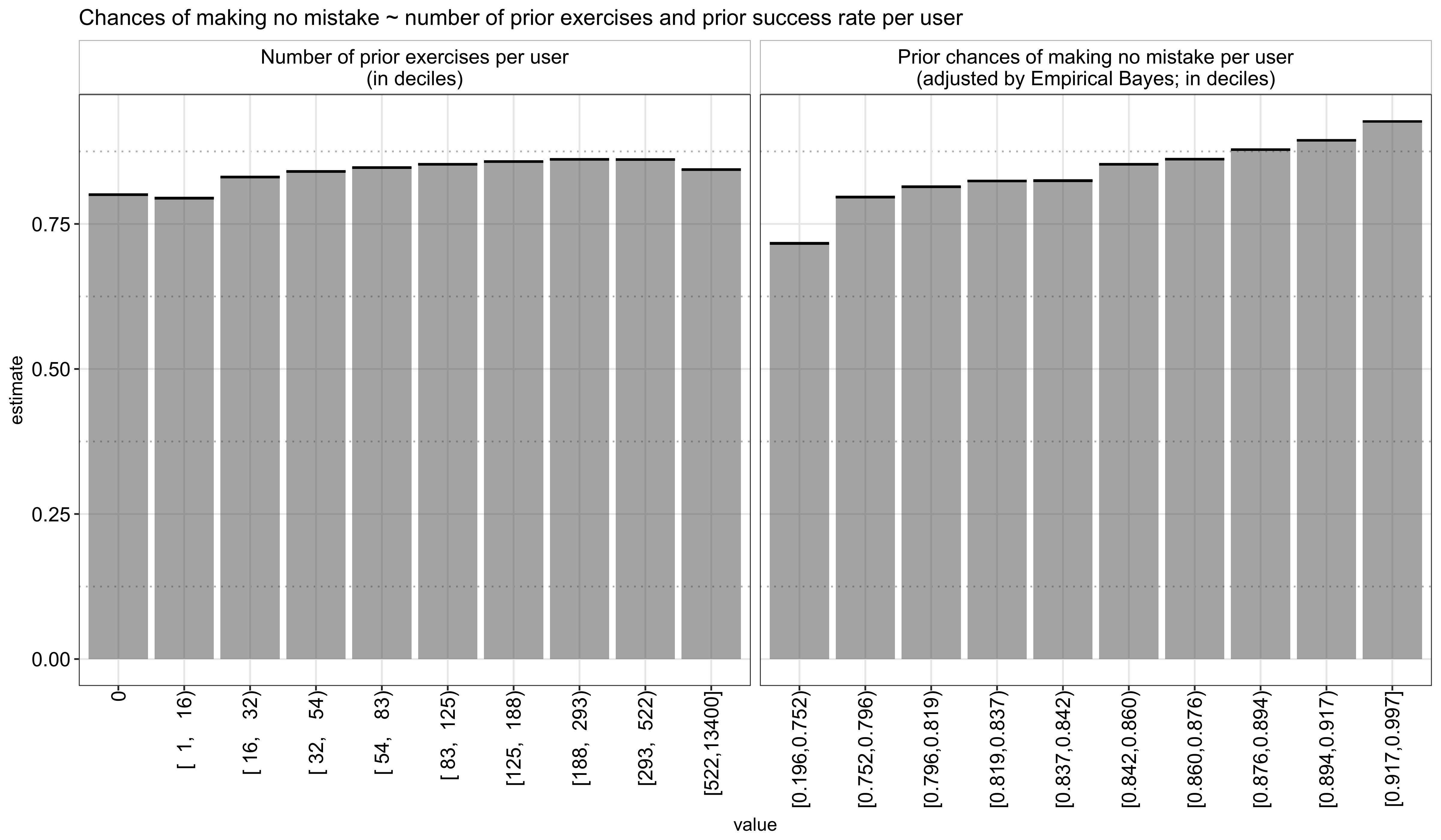
Using the prior number of exercises and the adjusted prior success rate, I analyzed how they impact a user’s performance in the current session and found that there is indeed an increasing relationship, particularly from the latter:
The users and the words
In the final section of the exploratory analysis, I’ll explore how a user’s past interaction with a given word impacts his/her ability of correctly recalling it in the current session.
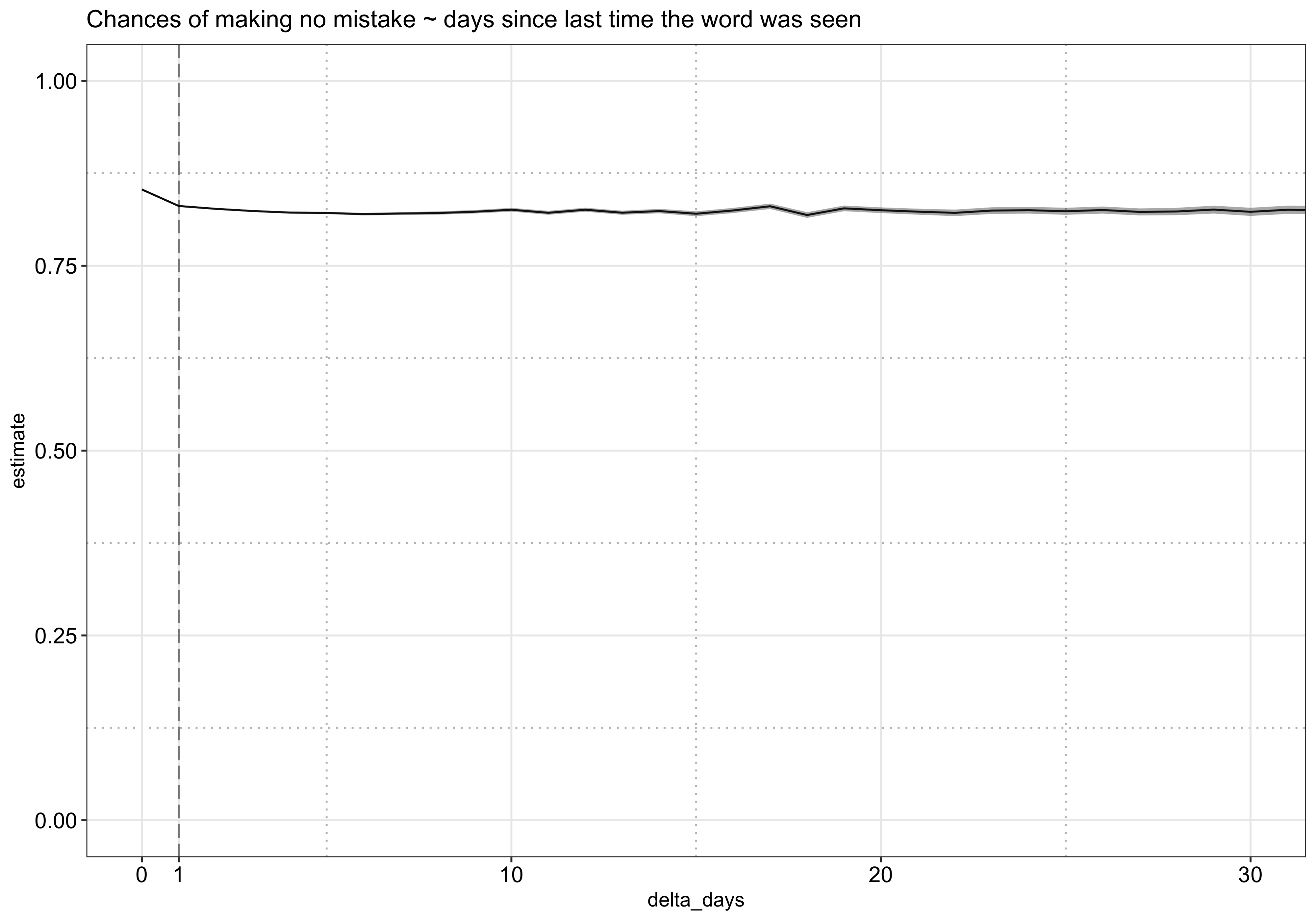
First, I analyzed how such ability declines with time. As shown in the plot below, there is a sharp drop at day 1 but remains rather flat afterwards. Note it is possible that this curve is influenced by Duolingo’s existing spaced-repetition algorithm at that time and does not reflect a user’s true forgetting curve (e.g., words that have not been shown for a long time might be the easy ones and have high success rates).
Next, I wanted to see how a user’s historical track record with a particular word impacts his/her current performance using the columns history_seen and history_correct. The former is straightforward,5 for the latter, I could use history_correct to compute the historical accuracy rate directly or use Empirical Bayes again to adjust the rate by incorporating the correct rate of all the words in a given language. I was a bit torn here because I can see the benefit from both sides: let’s say a person has only seen a word once before and has gotten it wrong, it might be harsh to assume his/her accuracy rate for this word is 0 but one can also argue we should show the word again soon given that he/she hasn’t had enough practice with it yet (to be conservative, we would use the unadjusted rate of 0 here); on the other hand, it is also hard to say if a score of 1 indicates true knowledge or simply luck (in this case, to be conservative, we would instead adjust it down to the global average). In this analysis, I opted to using the adjusted rate in the end but actually found the similar results using the unadjusted too.
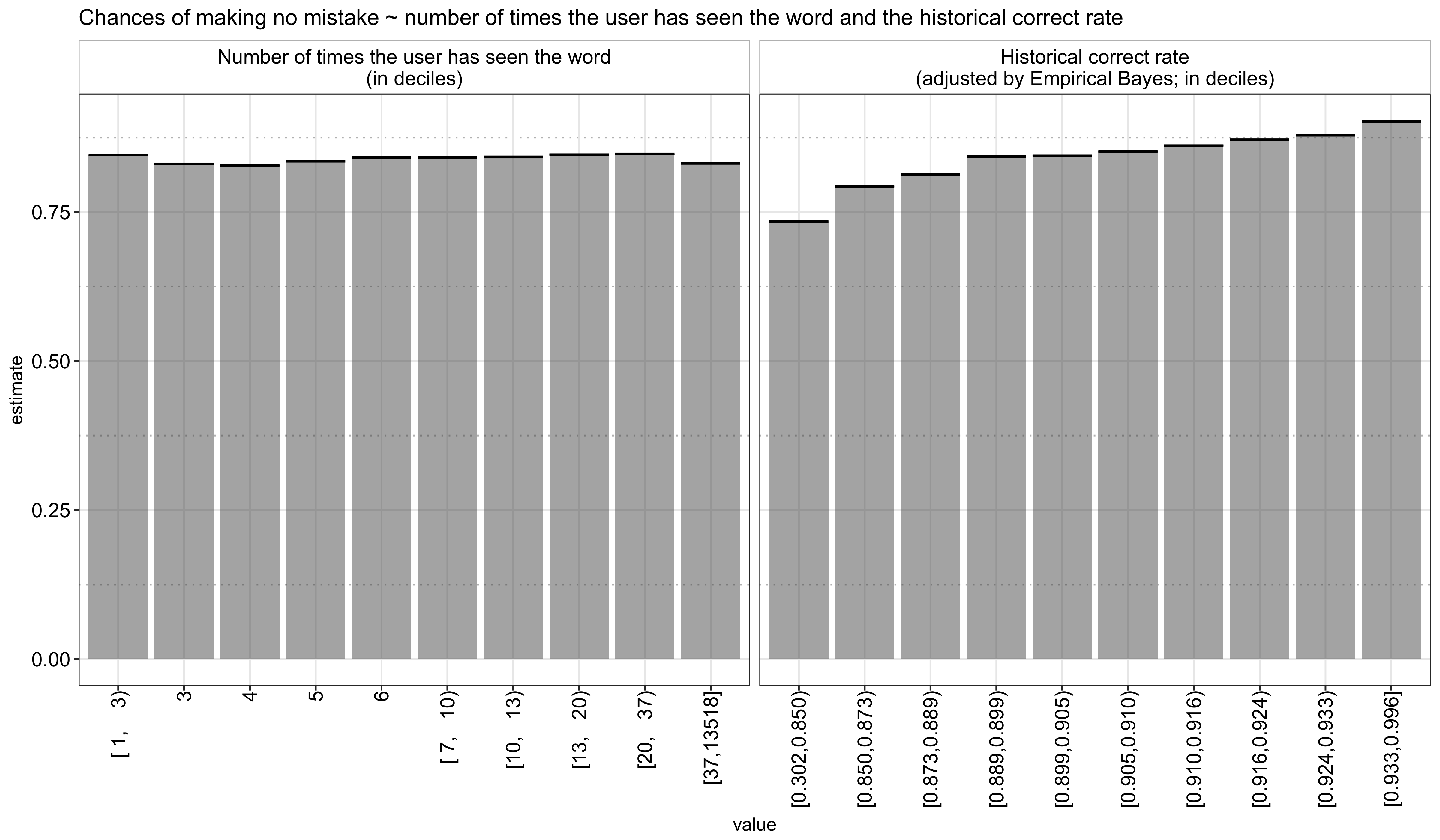
As shown below, the number of times a user has seen the word actually shows a slightly negative correlation with the current recall rate - this seemingly contradictory result may be because that Duolingo would repeatedly show a word if it has been shown difficult to remember for a given user. The historical correct rate, on the other hand, is more straightforward, that is, a user’s past ability to recall a word strongly correlates with his/her future performance on the same word:
Model training
Based on the exploratory analysis above, I extracted the following 9 features for model training:
ui_learning_language(ui_languageandlearning_languagepair)surface_form_lensurface_form_eq_lemma(whether asurface_formis exactly the same as itslemma)pos_binned(poswith the minority categories grouped together)log_prior_exercises_per_userprior_no_mistake_rate_per_userlog_delta_dayslog_history_seenhistory_correct_rate
As for the actual model, I tried a linear model (logistic regression) and a tree-based one (gradient boost trees):
# train models
## 5-fold cv
ctrl = trainControl(method = 'cv', number = 5, classProbs = T,
                    summaryFunction = twoClassSummary)

## logistic regression
duo_train_logit = train(x = duo_train_X, y = duo_train_Y,
                        method = 'glm', family = 'binomial',
                        metric = 'ROC', trControl = ctrl)

## ROC: 0.64

## gradient boost trees
duo_train_gbm = train(x = duo_train_X, y = duo_train_Y,
                      method = 'gbm', metric = 'ROC',
                      trControl = ctrl, verbose = F)

## ROC: 0.65
Based on cross-validation results, the two models show a similar performance in terms of AUC under ROC (0.64-0.65). Hence, I opted in for the simpler solution, logistic regression, in the end.
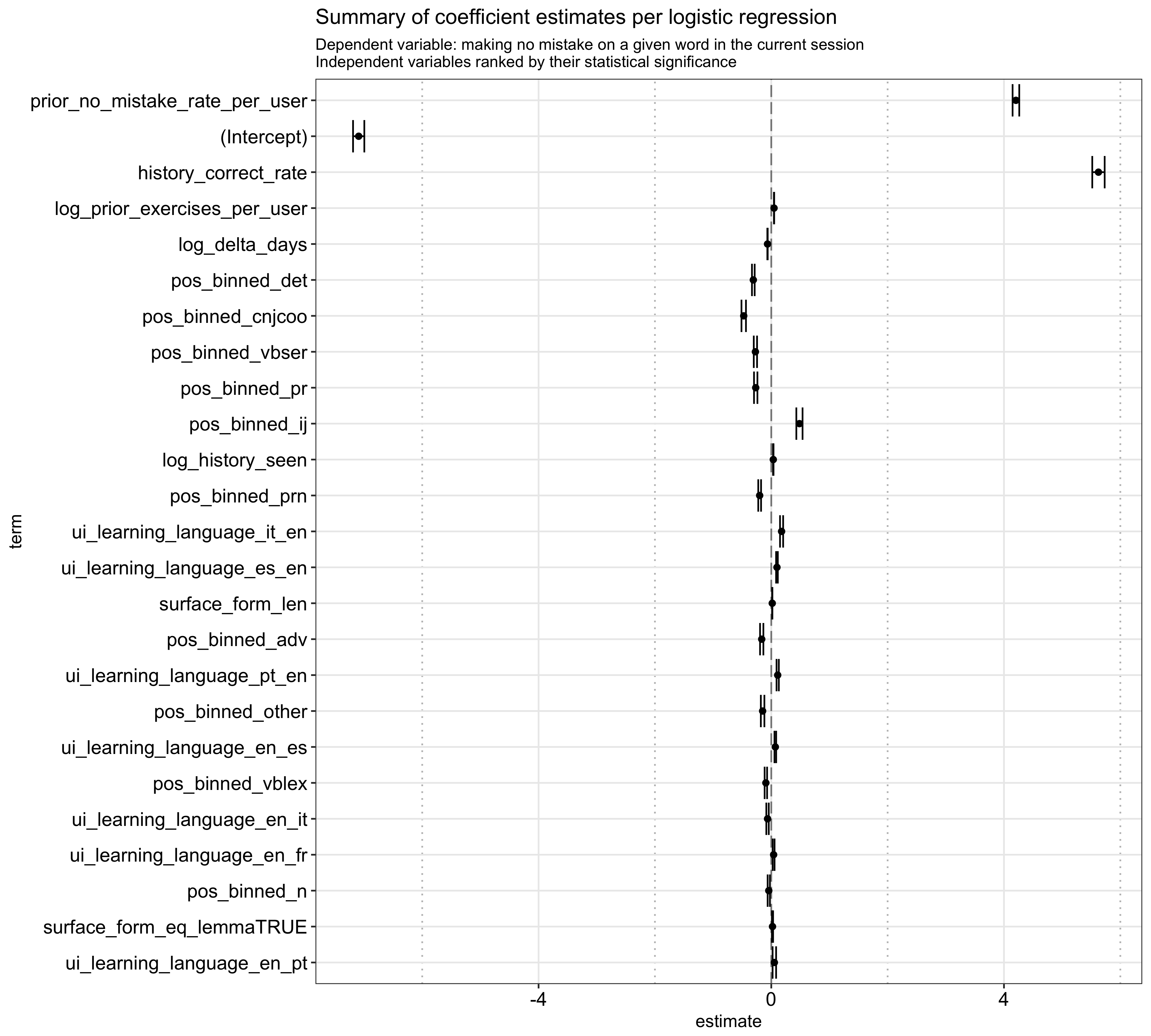
Besides the model performance, it is interesting to see the feature importance based on the statistical significance estimated by the logistic regression. As expected, the most important variables are a user’s prior success rate in general, his/her historical success rate for a given word in particular,6 the number of prior exercises he/she has completed, time since the word is last seen, and its part-of-speech tagging:7
Model testing
In this final section, I’m going to apply the trained model to the test data I set aside in the beginning to see how the model performs against it.
# apply the trained model
duo_test_no_mistake_pred = predict(duo_train_logit, newdata = duo_test_X, type = 'prob')
duo_test$no_mistake_pred = duo_test_no_mistake_pred$TRUE.
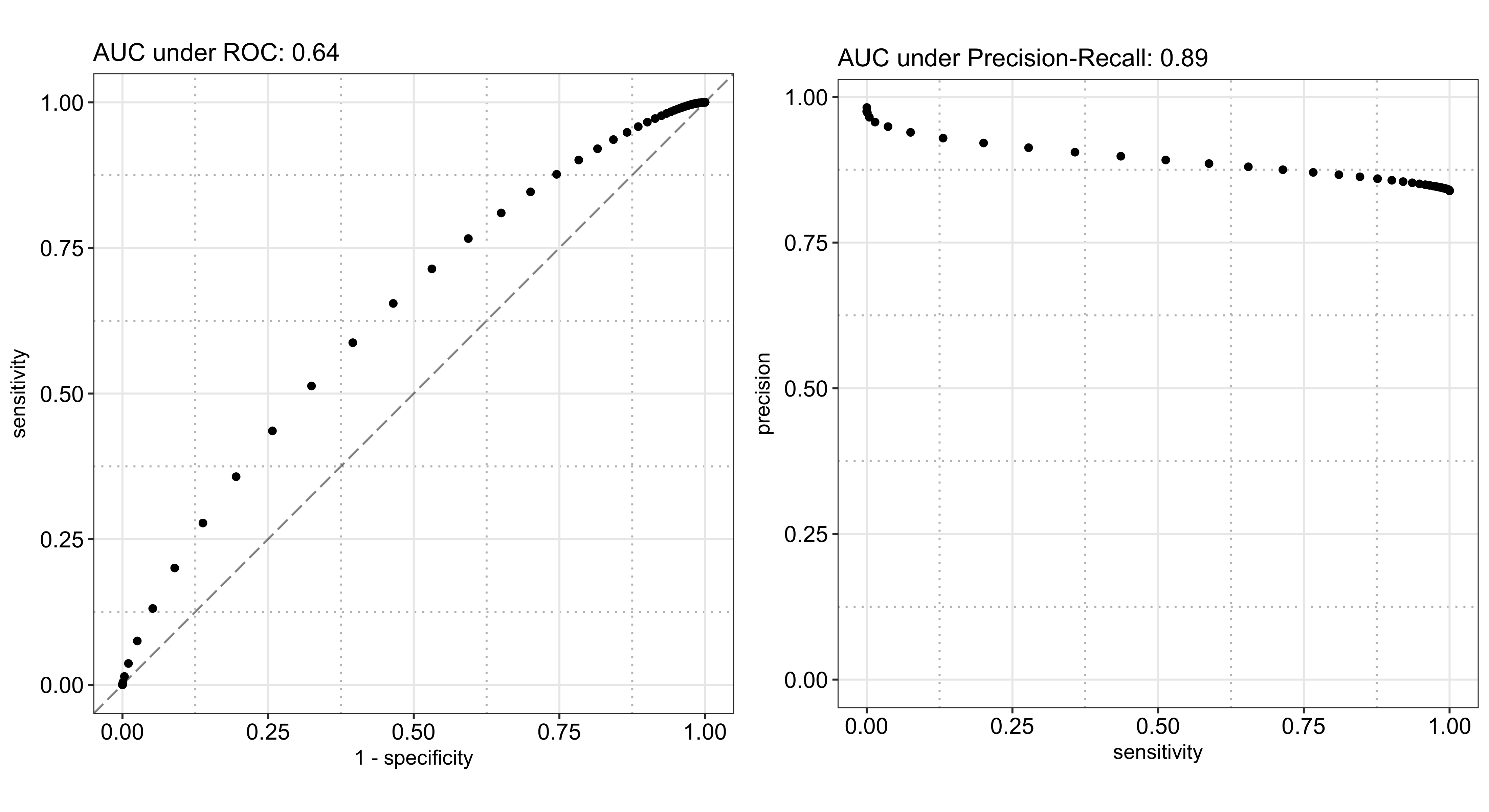
As illustrated below, the AUC under ROC is also 0.64, the same as the cross-validation result above, and the AUC under Precision-Recall is 0.89. The reason the latter is so high while the former is not so great is because 84% of the records have a positive outcome, which makes scoring a high precision ($P(\text{actually positive}|\text{predicted to be positive})$) and a high recall/sensitivity ($P(\text{predicted to be positive}|\text{actually positive})$) easy. In the most extreme case, if I just blindly predict every instance to be true, I would end up with a 100% recall rate and a 84% precision, which is still pretty good. However, in this case, it is hard to achieve a high specificity ($P(\text{predicted to be negative}|\text{actually negative})$) because the negative instances are rare,8 which drags the ROC down.
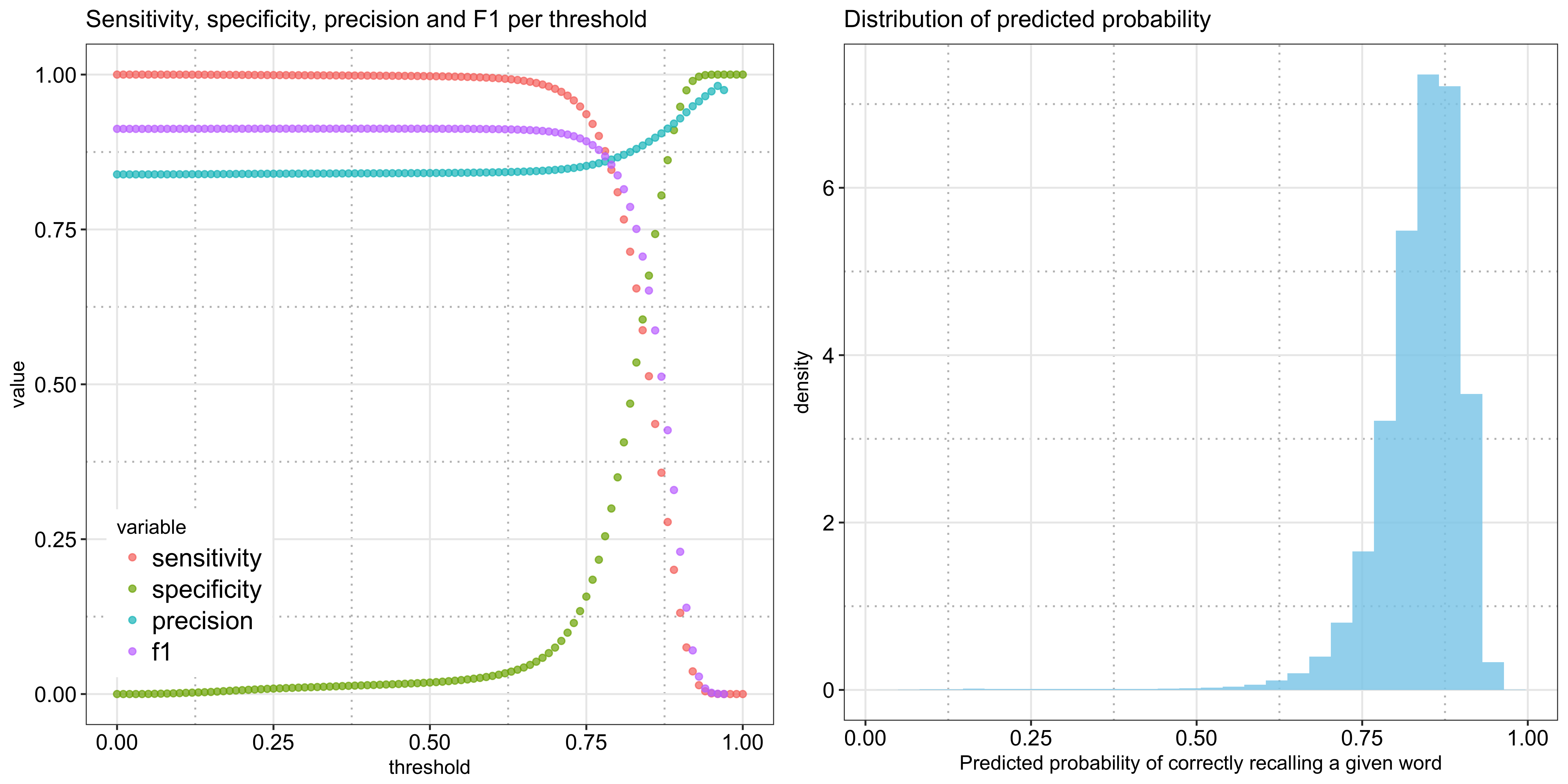
To illustrate the point further, the following plot shows the three metrics along with the F1 score per threshold - you can see how it takes a very high threshold for specificity to take off. Shown alongside is the distribution of the predicted probabilities, which is heavily left skewed due to the prevalence of the positive class and explains why the left plot stays rather flat for the lower values:
That said, instead of generating binary predictions, the model is perhaps more useful in ranking words given the finite number of words that can be shown in a lesson.
Future improvements
There is more we can do with the words themselves. For example, it would be interesting to examine the relationship between a word in the learning language with the words in the learners’ native languages to see if the similarity between the two help the users remember the word or not. The relationship may not be straightforward because, although Latin-based languages share many similar words, there are also a lot of “false friends.” If there is a scalable way to measure both the degree of being a “true friend” and a “false friend” for a given word, it may shed more light on understanding how one learns a foreign word and help predict the rate of correctly remembering it. Word similarity can measure the general similarity (e.g., Levenshtein distance), but it is blind to whether it is a true friend or not.
References
Settles, B., and B. Meeder. 2016. “A Trainable Spaced Repetition Model for Language Learning.” In Proceedings of the Association for Computational Linguistics (Acl), 1848–58. ACL.
David Robinson. 2017. Introduction to Empirical Bayes: Examples from Baseball Statistics. https://gumroad.com/l/empirical-bayes
- Without turning this post into a collection of language studying advice, the tools/resources I have tried and have found success in are (in addition to Duolingo) italki, Memrise, Readlang, TV5Monde, Speechling, Coffee Break French, Learn French with Alexa, and the classic French in Action series. [return]
- I also tried to only use features prior to a given session in my analysis, which means not using either
session_seenorsession_correct. [return] - 50 because based on the histogram, 50 per word is enough to create a smooth distribution. [return]
- Using only the data I have, I assume a user’s entire history is covered, which may not be true. [return]
- I noticed that the minimum of
history_seenis 1, indicating the first time a word is shown, i.e., the learning session, is removed. [return] prior_no_mistake_rate_per_userandhistory_correct_rateare not very correlated: the correlation is 0.38. [return]- The base level for
pos_binnedisadjand that forui_learning_languageisen_de. [return] - Also $P(\text{actually negative}|\text{predicted to be negative})$, although it’s not reflected in either curve. [return]