Background
Lately I’ve been spending a lot of time learning about deep learning, particularly its applications in natural language processing, a field I have been immensely interested in. Before deep learning, my foray into NLP has been mainly about sentiment analysis1 and topic modeling.2 These projects are fun but they are all limited in analyzing an existing corpus of text whereas I’m also interested in applications that generate texts themselves. While researching this topic, inevitably, I came across this famous blog post written by Andrej Karpathy that showcases the “unreasonable effectiveness” of recurrent neural networks (“RNN”) with models that output Shakespeare sonnets, Wikipedia articles, well-formatted LaTeX and source code, and even music notes! It is impossible not to get excited about this seemingly magic model and I was well motivated to learn more.
I had learned about the basic neural networks before but RNN was still new to me; I also needed to learn the new tools that have been developed for these purposes, so I took the quick Udacity’s deep learning class using TensorFlow.3 Overall, I highly recommend it but be aware that it is more of a hands-on course that focuses more on learning while doing and is sometimes rather light on theory. As a result, many times I got confused just by watching the video itself and had to resort to Google searches to really understand a concept. Honestly, this is not a bad process as it often helps by learning the same subject from different teachers, but just be prepared to put in the extra work from elsewhere (especially since the course is deceptively short). That said, one thing I especially appreciated about the class is its assignment code: not only is it ready to use and re-purpose, when explaining a specific network structure, it avoids using a pre-defined wrapper function - instead, it writes out all the steps behind the scene (at least the essential part), which helps you understand the theory better. Obviously in real life, you are more likely to call a high-level function directly, but being able to recall what’s really going on is arguably still better.
After finishing the class, I was eager to apply what I had learned to a project, particularly one that would use RNN to generate text as Karpathy did in that blog post. Because of my love for classical literature,4 I decided to train a model using the public Gutenberg data, which includes a large collection of books that are no longer under copyright protection and are hence free to download. Yet I don’t want to just use anyone’s work, so I decided to pick a few of my favorite authors, each with their own distinctive style, and mix them together. In the end, I settled on Jane Austen, Oscar Wilde, and F. Scott Fitzgerald, hoping my model would be able to pick up some of Austen’s sassiness (“I always deserve the best treatment because I never put up with any other.” - Emma), Wilde’s mischievous wittiness (“It is absurd to divide people into good and bad. People are either charming or tedious.” - Lady Windermere’s Fan), and Fitzgerald’s beautiful melancholy (“So we beat on, boats against the current, borne back ceaselessly into the past.” - The Great Gatsby).
In the following sections, I’m going to detail my methodology, from data collection to model training. It was one of my favorite projects and I hope my passion is able to make the remaining post fun to read :-)
Downloading and pre-processing data
I could’ve downloaded the raw Gutenberg data directly but David Robinson has a very handy R package called gutenbergr which allows me to look up and download multiple works at the same time with ease. It also returns data in a tidy format, which makes the pre-processing a joy too.
I’ll go through this section quickly (you can find the entire code here): first I downloaded all the works by the three authors in one batch using gutenberg_download:
# Select books to download
# (stored in pre-defined dataframes `oscar_wilde`, `jane_austen`, and `f_scott_fitzgerald`)
works_to_download = oscar_wilde %>%
  bind_rows(jane_austen) %>%
  bind_rows(f_scott_fitzgerald)

# Download
works = gutenberg_download(works_to_download$gutenberg_id, meta_fields = 'title')
This returns a tidy dataframe with the text broken arbitrarily into rows. Ultimately, I need to feed a sequence of words broken out individually to TensorFlow, which I can achieve by applying the unnest_tokens function from Julia Silge and David Robinson’s tidytext package.5 However, before I do that, I need to decide where to split the whole text into training, validation, and test sets. The easiest way would be to cut the chain of words themselves into three portions, but I tried to avoid doing that because I didn’t want to break the sequence of a running theme, which I was hoping RNN, a sequential model, would be able to learn. Hence, instead I first broke the text into paragraphs and keep the corpus intact within a paragraph and only split it in between. By so doing, I hope a nice running sequence is not badly interrupted.
# Break into paragraphs
works_paragraphs = works %>%
  unnest_tokens(paragraph, text, token = 'paragraphs')

# Additional processing omitted...
# Seperate paragraphs into training, validation, and testing on a per-title basis
works_paragraphs = works_paragraphs %>%
  group_by(title) %>%
  mutate(rn = row_number(),
         n = n(),
         grp = ifelse(rn / n <= .8, 'train', ifelse(rn / n <= .9, 'valid', 'test')))
With some additional processing (e.g., converting punctuation marks to words so that tidytext would not remove them), I was finally able to safely break paragraphs into words and pass them on.
Aside from this initial processing, the rest of the analysis is done in Python with code adapted from this TensorFlow tutorial and an extension contributed by this blog post. My code is written in a Jupyter Notebook and is hosted here.
It is true that, given the amount of code I’m reusing (or stealing) from the tutorial, I could have simply pointed to the original and skipped the lengthy explanation, but a big part of the reason that I chose to still go through it here is to help myself understand it better by trying to explain it, in my own words, to my imaginary friend, so bear with me :-)
Before feeding words directly into the model, to make the processing easy, it is better to first convert each word to a unique identifier. The following snippet does that by using each word’s frequency as its identifier and creating mappings for both directions (note there are about 38,000 unique words in our data, which is our vocab_size):
# Create word-to-ID mapping
counter = collections.Counter(data['word'])
count_pairs = sorted(counter.items(), key=lambda x: (-x[1], x[0]))

words, _ = list(zip(*count_pairs))
word_to_id = dict(zip(words, range(len(words))))
id_to_word = dict(zip(range(len(words)), words))

vocab_size = len(word_to_id)
vocab_size  # 38115
Next, I split the word IDs into training, validation, and test sets as defined in the R code above:
# Separate data into training, valid, and testing
train_data = [word_to_id[w] for w in list(data['word'][data['grp'] == 'train'])]
valid_data = [word_to_id[w] for w in list(data['word'][data['grp'] == 'valid'])]
test_data = [word_to_id[w] for w in list(data['word'][data['grp'] == 'test'])]

len(train_data), len(valid_data), len(test_data)
# (1842988, 206542, 218819)
The basics of RNN and LSTM
To understand RNN and its extension, Long Short Term Memory (“LSTM”), the single best resource I have found is this blog post written by Christopher Olah. Instead of repeating what Olah has explained so eloquently, I’ll just summarize the key ideas below based on my understanding.
At its core, RNN is a sequential model, meaning that its input has a meaningful sequence that should be kept the same when feeding into the model. In this project, I am training a word-based model so each word in a sequence is inputted as a training data point, with the next word used as the targeting label. Using the famous opening line from The Great Gatsby, “in my younger and more vulnerable years my father gave me some advice that I’ve been turning over in my mind ever since,” the process looks like this:
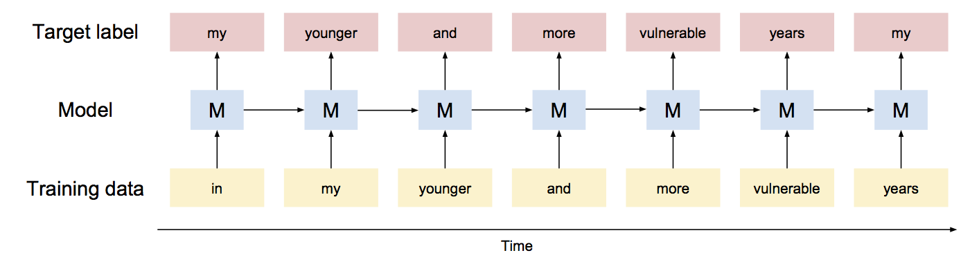
Note each model unit takes input from both the current word and the previous unit. Specifically, the input from the previous model unit is called the cell state, which can be thought of as the accumulated memory of what has been fed so far (e.g., the subject pronoun, the verb, the open quote) and is the key reason why RNN is able to remember contexts and syntaxes and, thus, able to generate meaningful sentences. Without memory, the model can still generate texts simply based on the previous word only, but it would be hardly meaningful.
Another key idea of RNN is using shared weights across time. Even though when you “unroll” an RNN, there are multiple model units connected with each other (i.e., each “M” in the illustration above), each of them actually share the same weights. This is similar to Convolutional Neural Networks (“CNN”), which shares weights across space as it is applied to image recognition.
However, because RNN shares weights, during its backpropagation process, we are applying all these derivatives to the same parameters, which creates a lot of correlated updates and may result in exploding gradients and vanishing gradients. To prevent exploding gradients, we can simply apply a cap to all gradients; to prevent the vanishing problem, which makes it hard for the model to remember the previous information, we can replace the plain RNN unit with LSTM, which helps the model keep its memory longer when it needs to, and ignore things when it should.
Olah’s post has an excellent section that walks through each component of LSTM step by step. Here, I’ll just summarize the key steps:
When new information comes in (e.g., a new word), LSTM first uses it to decide which part of the stored information (i.e., the previous cell state) is no longer relevant (e.g., an old subject pronoun) and constructs a forget gate by wrapping a sigmoid function around this new input (along with the previous prediction output) so that the resulting values range from 0 to 1. It then applies the forget gate to each value in the cell state in a pointwise multiplication to selectively forgets (if a value from the forget gate is 0) and remembers them (if it’s above 1).
After deciding what to forget, the model also needs to decide what new information to store, and it does so by applying another sigmoid function, known as the input gate, to the input (along with the previous output) so that the result is a filtered version of the input.
Next, it updates the cell state by removing the information the forget gate decides to forget and adding the new information the input gate decides to add.
Finally, it needs to decide what to output based on the cell state that was just updated by applying another sigmoid function to it (It doesn’t need to output all the accumulated information so far because not all of them may be relevant to what is coming next). This output is then compared with the target label (e.g., the next word) to compute losses, which are later minimized using gradient descent.
Obviously, this is a very high-level overview. To understand what goes behind the scene, I recommend reading this sample code in Udacity’s assignment, where, instead of calling the wrapper function tf.contrib.rnn.BasicLSTMCell, it writes out a basic LSTM cell itself, including the entire updating process explained above. It certainly helped me a lot to combine the high-level intuition with the actual implementation.
Generating batches
With the model structure in mind, I’m going to demonstrate the key steps of building an RNN model with the LSTM cells below, again using code adapted from TensorFlow’s tutorial linked above.
Instead of feeding the entire training data to the model all at once, to speed up the process, we can use stochastic gradient descent by feeding a small random sample at a time. Each sample is called a batch and its size is determined by the hyperparameter batch_size. In my implementation, I set batch_size to be 20, so I’m feeding 20 word sequences at a time.
The length of each sequence is defined by another parameter called num_steps.6 Here I set num_steps to be 35, so each sequence has exactly 35 words in it. The length of the sequence is a trade-off: if it’s too short, the model doesn’t have enough information to predict the next word; if it’s too long, the model needs to carry a lot of unnecessary information that is not relevant anymore. However, LSTM, with its selective update, is able to mitigate the latter problem.
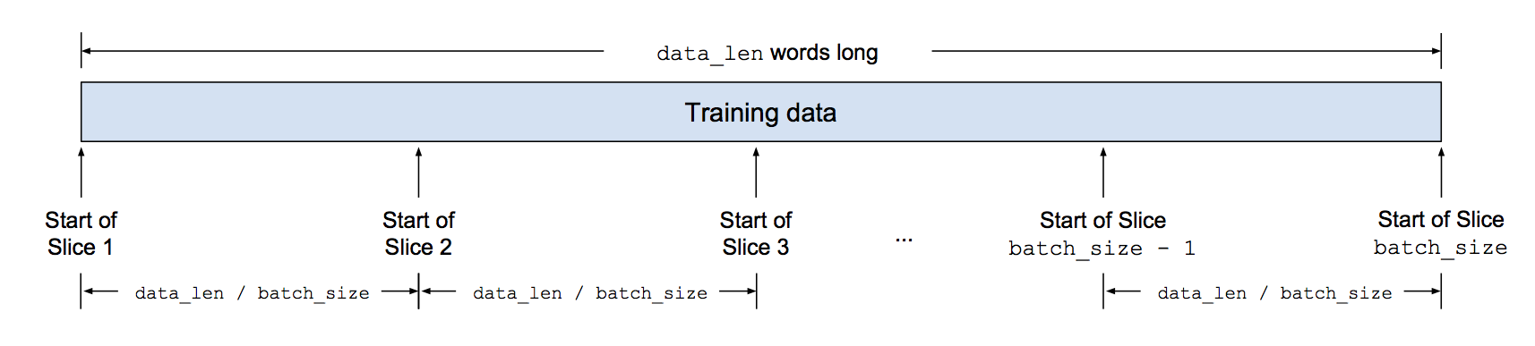
To demonstrate the whole batch producing process,
- Suppose our training data has
data_lenwords, to generate a batch ofbatch_sizesequences at a time and make sure they don’t overlap, we can slice the data intodata_len / batch_sizeslices and generate sequences that aredata_len / batch_sizewords apart:
- After spliting the raw data into slices, it is useful to know how many sequences we can generate in total within each slice. Since the length of each sequence is
num_steps, the answer is(data_len / batch_size) / num_steps, known asepoch_size:
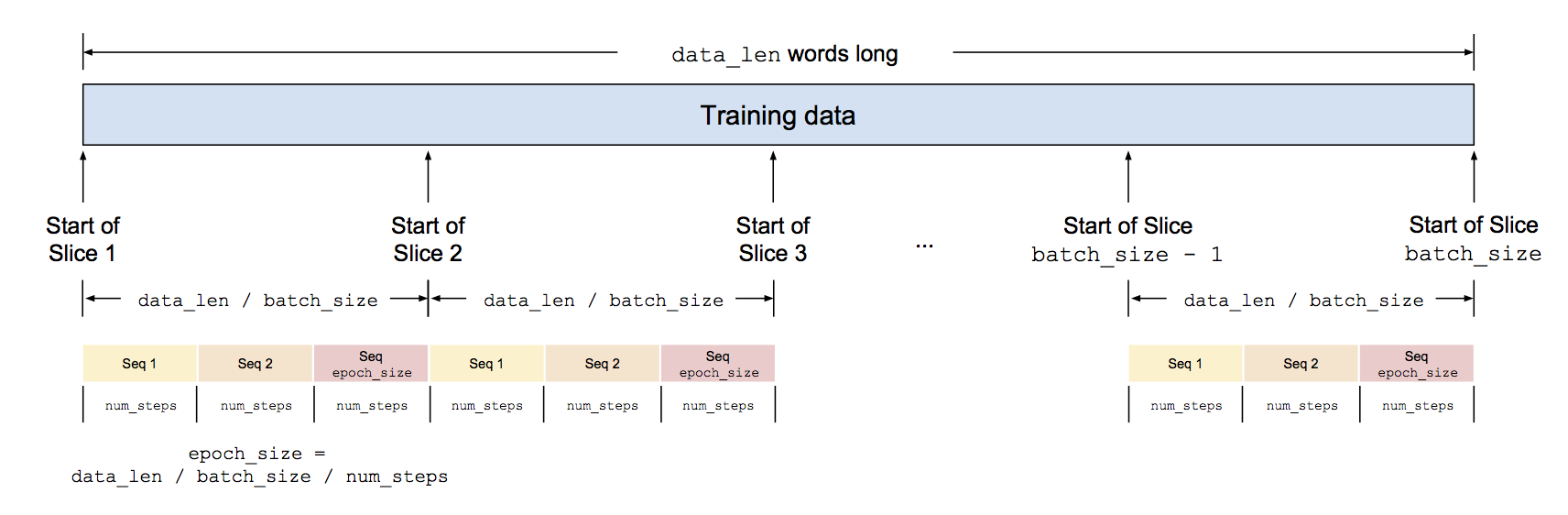
The reason the number of sequences inside a batch is called
epoch_sizeis that the number of iterations it takes to go through our entire training set is called an epoch. Imagine in the beginning of the first iteration, our cursors are at the start of each slices. Then at each iteration, we make a strike ofnum_stepslong, and it will take usepoch_sizeiterations to finish feeding all the training data into our model.There is just one snag though: as demonstrated in the first diagram above, we shift the training data by one word to create the target labels. If we use the hyperparameters defined above, we may run into the risk of not having a label for the last training word. Hence, to prevent this situation, we drop the last word when computing
epoch_size, so instead of(data_len / batch_size) / num_steps, we do(data_len / batch_size - 1) / num_steps.
To summarize, at a given iteration, our input data to the model is of shape [batch_size, num_steps] (so is our label data), and we iterate (data_len / batch_size - 1) / num_steps times to cover the entire dataset.
In the code, this process is defined in a function called batch_producer and is used to create a model input object (defined in class ModelInput), including input_data, targets, and such hyperparameters as batch_size and epoch_size.
Defining model
In this section, I’m going to go through the key components in defining the model.
Word embeddings
Without doing anything, our input data right now is a sequence of word IDs that have vocab_size unique values. If we apply one-hot encoding to them and feed the resulting matrix to the model, it is very inefficient and resource-intensive. A common solution is to convert each word into a dense vector called word embedding and feed them into the model instead.
Word embedding is a very interesting topic in itself, and Google’s word2vec is a famous implementation of the idea and is able to produce meaningful word vectors such that words with similar meanings are close to each other in cosine distance (e.g., although “dog” and “puppy” are spelled very differently and no character-based encoding would be able to group them together, the vectors produced by word2vec are able to). Despite its magic-like results, the theory behind is actually very simple: for a given word input (e.g., “dog”), the model first initializes a random embedding for it. Then it takes the whole context this word appears in (e.g., “dog barks”) and trains a model to predict its adjacent words one by one (e.g., “dog” -> “barks”). Meanwhile, if there is another word that tends to appear in the same context (e.g., “puppy” as in “puppy barks”), in order to achieve high accuracy in predicting this same context (e.g., “barks”), the model is motivated to optimize the the two words’ embeddings in such a way that the resulting vectors are highly similar to each other.7
In our RNN model, although the objective function is different, we can still borrow the idea of embeddings to reduce dimensions. The desired embedding size is determined by the parameter hidden_size and, in my project, I set it to 256. It’s called hidden_size because it also defines the number of hidden units outputted by each LSTM cell, so without adding another hidden layer, we simply set the embedding size equal to the size of the hidden units.
Recall our input data is of shape [batch_size, num_steps]. After mapping each word to a embedding of length hidden_size, the shape becomes [batch_size, num_steps, hidden_size].
embedding = tf.get_variable("embedding", [vocab_size, hidden_size], dtype=tf.float32)
input_embeddings = tf.nn.embedding_lookup(embedding, input_data)
Dropout
Dropout is a regularization technique that randomly sets a portion of the activation nodes to 0, thereby forcing the remaining nodes to learn on their own of sometimes the redundant information, eventually making the network more robust and preventing overfitting. After training, because there are multiple nodes that were trained to learn the same thing, a consensus is generated by averaging the outputs. The idea is very similar to ensemble learning.
In the code, we first add dropout to the input embeddings based on pre-defined keep_prob (Note we only implement dropout in the training process, not in validation or testing):
# Implement dropout to input embedding data
if is_training and keep_prob < 1:
  input_embeddings = tf.nn.dropout(input_embeddings, keep_prob)
Then, we also add dropout to the outputs of the LSTM cells. Assuming we have already defined a basic LSTM cell using tf.contrib.rnn.BasicLSTMCell, we can simply call tf.contrib.rnn.DropoutWrapper:
# Implement dropout to the outputs of LSTM cells
if is_training and keep_prob < 1:
  def attn_cell():
    return tf.contrib.rnn.DropoutWrapper(lstm_cell(), output_keep_prob=keep_prob)
Stacking multiple LSTMs
To improve model performance, we can stack multiple LSTM cells together so that the output of the previous one becomes the input of the next. The number of layers is determined by num_layers and I set it to 2 in my implementation. In TensorFlow, we can call tf.contrib.rnn.MultiRNNCell to do that:
# Stacking multiple LSTMs
attn_cells = [attn_cell() for _ in range(num_layers)]  # attn_cell() is a single-layer LSTM cell
stacked_lstm = tf.contrib.rnn.MultiRNNCell(attn_cells, state_is_tuple=True)
Note we set state_is_tuple=True in defining multiple LSTMs, and it’s simply saying that the output, namely, the new cell state and cell output (also known as the hidden state), is returned in a tuple (i.e., (cell_state, cell_output)).
Unrolling LSTM
Next, using this stacked LSTM, we feed one word to it at a time as described above. This process is called unrolling. The essential code is like this:
outputs = []

# Initialize states with zeros
initial_state = stacked_lstm.zero_state(batch_size, tf.float32)
state = initial_state

for time_step in range(num_steps):
  # Recall that `input_embeddings` is shaped [batch_size, num_steps, hidden_size]
  (cell_output, state) = stacked_lstm(input_embeddings[:, time_step, :], state)
  outputs.append(cell_output)
Note stacked_lstm returns a tuple of (cell_output, state), where state itself is a tuple of (cell_state, cell_output) (as explained previously) so the return value is (cell_output, (cell_state, cell_output)). state is fed to the next cell unit as the previous state while the cell_output is saved separately in a list called outputs, which is going to be compared with the target labels later. This process continues until we finish processing all the words in a word sequence.
Computing output logits
For each output produced by a LSTM cell, shaped [batch_size, hidden_size], in order to compare with the target label to compute loss, we produce a logit that is shaped [batch_size, vocab_size], by multiplying a weight matrix shaped [hidden_size, vocab_size]. Because the output we produced above (i.e., outputs) is a list of num_steps elements, we need to first resize it into a two-dimensional matrix:
# Resize the ouput into a [batch_size * num_steps, hidden_size] matrix.
output = tf.reshape(tf.stack(axis=1, values=outputs), [-1, hidden_size])

# Compute logits
softmax_w = tf.get_variable("softmax_w", [hidden_size, vocab_size], dtype=tf.float32)
softmax_b = tf.get_variable("softmax_b", [vocab_size], dtype=tf.float32)

logits = tf.matmul(output, softmax_w) + softmax_b
# The resulting shape of `logits` is [batch_size * num_steps, vocab_size]
This so far is good enough to compute losses and evaluate against the validation and test sets, but to generate text, which is our ultimate goal, we need to add a sampling function here that returns an actual word as the prediction and the input to the next one. This is realized by calling the tf.multinomial function, which draws samples from a multinomial distribution based on the size of the different logit outputs (i.e., the higher the prediction value for a given word is, the more likely the function is going to select it):
logits_sample = tf.multinomial(logits, 1)
Note the reason we sample instead of always taking the word with the largest logit value (by using np.argmax(logits)) is that we want to introduce some randomness to the result instead of running into the risk of always using the same word after another.
Computing the loss function
To compute loss between predictions and target labels, we call tf.contrib.seq2seq.sequence_loss that computes cross-entropy loss for a sequence of logits:
# Reshape logits to be 3-D tensor for sequence loss
logits = tf.reshape(logits, [batch_size, num_steps, vocab_size])

loss = tf.contrib.seq2seq.sequence_loss(
  logits,  # shape: [batch_size, num_steps, vocab_size]
  targets,  # shape: [batch_size, num_steps]; represents the true class at each step
  tf.ones([batch_size, num_steps], dtype=tf.float32),  # weights (all set to 1 here)
  average_across_timesteps=False,
  average_across_batch=True)

# Compute the total loss and update the cost variables
cost = tf.reduce_sum(loss)
Optimizing using gradient descent
First, we need to initialize the optimizer using tf.train.GradientDescentOptimizer, which requires us to specify a learning rate:
optimizer = tf.train.GradientDescentOptimizer(learning_rate)
As mentioned in TensorFlow’s website, “when training a model, it is often recommended to lower the learning rate as the training progresses,” and normally we can just call the tf.train.exponential_decay function directly to specify the initial learning rate, decay steps, and decay rate. However, in this tutorial code that I adapted, it decided to have more control over how learning rate decays and chose to update it itself when running the model (as we’ll see later on). Regardless, the idea is the same.
Next, we compute gradients of the cost with respect to all the trainable variables (e.g, weights, embeddings):
tvars = tf.trainable_variables()  # this literally returns all trainable variables in a list
grads = tf.gradients(cost, tvars)  # compute partial derivatives of `cost` w.r.t. each `tvars`
grads, _ = tf.clip_by_global_norm(grads, max_grad_norm)  # cap gradients at `max_grad_norm` to prevent them from exploding
Finally, we apply the gradients to trainable variable using apply_gradients():
global_step = tf.contrib.framework.get_or_create_global_step()
optimizer = optimizer.apply_gradients(zip(grads, tvars), global_step=global_step)
This concludes the model definition process. In the code, these steps are defined in class Model and executed when a session.run is called.
Running an epoch
Recall that during an epoch, we feed the entire input data, batches by batches, into the model, and it takes epoch_size iterations to complete. While in an epoch, the costs and states are not reset and are accumulated until the end. Only at the start of the next epoch do they get reset again.
The steps of running an epoch are defined in function run_epoch and are executed in a running session. Here I’ll just go through some key steps below:
Initializing costs and states
The following snippet initializes costs to 0 and returns the zero initial_state:
# Initialize costs to 0
costs = 0.0

# Initialize state values to 0s
# In class `Model`, states are initialized to 0s using:
# `initial_state = stacked_lstm.zero_state(batch_size, tf.float32)`
state = session.run(model.initial_state)

# Initialize counter to  0
# To be used to compute average cost later
iters = 0
Next, we determine what we want to retrieve from the model after each successful run of a batch: for all sessions, we retrieve the final cost and state to update the current values; for training sessions, we also retrieve the optimizer object to trigger gradient descent.
# Determine what to return from each iteration
# These become the starting costs and states for the next iteration
fetches = {
  "cost": model.cost,
  "final_state": model.final_state,
}

# If in a training session, also return `optimizer` to trigger gradient descent
if optimizer is not None:
  fetches["optimizer"] = optimizer
Iterating through an epoch
After initialization, we start the iteration, one epoch_size at a time, to scan through the whole dataset and feed it to the model sequentially:
for step in range(model.input.epoch_size):
  # To update state values
  feed_dict = {}

  # Recall that `initial_state` is a list of `num_layers` tensors
  # Each is a tuple of (`c_state`, `h_state`)
  for i, (c, h) in enumerate(model.initial_state):
    feed_dict[c] = state[i].c
    feed_dict[h] = state[i].h

  # Kick off a session run with new states
  vals = session.run(fetches, feed_dict)

  # Upon finishing, extract cost and final_state after the current step,
  # which become the new initial cost and state for the next step
  cost = vals["cost"]
  state = vals["final_state"]

  # Compute average cost up to the current step
  costs += cost
  iters += model.input.num_steps
  perplexity = np.exp(costs / iters)
When I first read this part in the tutorial code, I was very confused as to how states are updated and how data is fed into the model. After a lot of Google searches, I now have a better understanding. I’ll try to explain it here in case you have the same questions:
We mentioned above that, in class Model, we initialize initial_state to be all 0s - what we really did there is initialize a list of num_layers tuples, (cell_state, cell_output), to 0s, so when we enumerate this list here, we are fetching the tuples one by one and putting them temporarily in (c, h).8
Then, we use feed_dict to tell the model in the next run to replace these initial values with the new ones stored in state, which are the previous final_state that we requested the model to return.9 It’s a bit confusing here because state is a named tuple whose names are also c and h, and they have nothing to do with the initial state tuple (c, h) that are returned from enumerate.
As for how batches are fed into the model, I was confused at first because, in all Udacity’s assignments, they are fed through feed_dict into a tf.placeholder object that is declared when defining the model graph. However, in this tutorial code, feed_dict only includes state updates, so how does the model receive the data?
It turns out that, in the function to generate batches, we defined a queue using the following code:
# From function `batch_producer`
i = tf.train.range_input_producer(epoch_size, shuffle=False).dequeue()

x = tf.strided_slice(data, [0, i * num_steps], [batch_size, (i + 1) * num_steps])
x.set_shape([batch_size, num_steps])

y = tf.strided_slice(data, [0, i * num_steps + 1], [batch_size, (i + 1) * num_steps + 1])
y.set_shape([batch_size, num_steps])
Before going into the detail of tf.train.range_input_producer, let’s first just assume it’s a sequence number ranging from 0 to epoch_size - 1, and imagine there is a for loop somewhere that uses it to slice data to produce x and y, the training input and the target labels, iteratively. Even though tf.strided_slice is a TensorFlow function, it’s equivalent to Numpy’s indexing and all it does is to carve out a sequence of length num_steps from each slice.10
But how does tf.train.range_input_producer(epoch_size, shuffle=False).dequeue() really work? There is no such a for loop in function run_epoch. it turns out the dequeue() operation, as well as the subsequent slicing, is triggered whenever a session is kicked off (e.g., using session.run as in run_epoch) that demands a return value involving a data operation. To illustrate the point, in run_epoch, there are two places where we trigger a session.run:
# Initialization
state = session.run(model.initial_state)
# ...

# Iterate over `epoch_size`
for step in range(model.input.epoch_size):
  # ...
  vals = session.run(fetches, feed_dict)
In the first place above, we trigger a session run to return the initial state and because, for the model to compute and return this value, it doesn’t need any actual input data (all it needs to do is set everything to 0), the dequeue() operation is not triggered, meaning our cursors have not moved.
In the second place, we ask the model to return fetches, which is a dictionary of cost and final_state, and to do that, the model has to actually find the input data and set RNN to run. Hence, in this case, dequeue() is triggered, data is sliced, and the cursors have moved.
To summarize, the model is defined with an input data object, which includes a queue of word sequences ready to be fed into the model whenever a session that requires them is kicked off.
Generating text
The last piece we need to implement before putting everything together is to generate text. This part is omitted from the original tutorial code and my implementation is based on this very helpful blog post. The function is very similar to run_epoch in structure with a few exceptions:
First of all, we need the model to return the logits_sample value to use as the prediction and the input to the next iteration, so we add that to our wishlist fetches:11
fetches = {
  "final_state": model.final_state,
  "logit_sample": model.logits_sample
}
Next, we choose a seed word for the model to start with and define the length of the text we want to generate. In my implementation, I tried various subject pronouns as the seed and chose to output a text of 500 words:
# Use various pronouns as the start of each text
feeds = ['he', 'she', 'it', 'mr', 'mrs', 'miss']
feeds = [word_to_id[w] for w in feeds]

# Define sentence length
text_length = 500
To pass the seed and the subsequent predictions into the model, we can’t use a pre-defined data object anymore because we don’t have a sequence yet - it’s what we are trying to generate! Hence, in this case, we’ll have to rely on feed_dict to send words into the model one at a time:
# `feed` is the seed word and is the beginning of the text to be generated
generated_text = [feed]

for i in range(text_length):
  feed_dict = {}
  feed_dict[model.input_data] = feed

  for i, (c, h) in enumerate(model.initial_state):
    feed_dict[c] = state[i].c
    feed_dict[h] = state[i].h

  vals = session.run(fetches, feed_dict)

  # Extract final state and sampled logit after the current step,
  # which become the new initial state and feed for the next step
  state = vals["final_state"]
  feed = vals["logit_sample"]

  # Append generated text
  generated_text.append(feed)
Note because we are feeding a single word at a time instead of a word sequence like we do in training, we don’t need multiple LSTM units anymore, so in the configuration, we set num_steps to 1. However, it doesn’t mean the model only makes predictions based on one word only. As shown in the snippet above, it still keeps a cumulative state object until an epoch is completed.
Putting it all together
With everything in place, we are ready to run it all! Like all TensorFlow models, we need to first define a model graph. To save space, I’m only including the definition of the training model, which is reused for validation, test, and text-generation purposes, and the text-generation model here:
with tf.Graph().as_default():
  # Initializer to initialize all variables defined in the `Model` object
  initializer = tf.random_uniform_initializer(-init_scale, init_scale)

  # Define training model using training data
  with tf.name_scope("Train"):
    train_input = ModelInput(config=config, data=train_data, name="TrainInput")
    with tf.variable_scope("Model", reuse=None, initializer=initializer):
      m = Model(is_training=True, config=config, input_=train_input)

  # Omitting models for validation and testing...

  # Define model for text generations (reusing training model)
  # No input data given here as we are going to dynamically generate input later
  with tf.name_scope("Feed"):
    with tf.variable_scope("Model", reuse=True, initializer=initializer):
      mfeed = Model(is_training=False, config=eval_config)
In short, the initializer object is used to initialize all variables defined in the model (e.g., weights, embeddings) using a uniform distribution in a pre-defined scale. Compared to the training model object m, the text-generation model mfeed is told to reuse the training model (i.e., reusing the trained weights, biases, etc.) and is defined without a train_input because, aside from the seed word, we are creating it on the fly. Also it is given a different config object because we set both batch_size and num_steps to 1.
Next, we open a session and call run_epoch to set things to run. In the code below, there are two badly-named hyperparameters: max_max_epoch and max_epoch, and they refer to the total number of epoch we want to run and the number of epoch we want to wait until we start decaying learning rate. In my implementation, I set them to be 20 and 6, respectively.
sv = tf.train.Supervisor(logdir=save_path)
  with sv.managed_session() as session:
    for i in range(max_max_epoch):
      # Update learning_rate if `i` >= `max_epoch`
      lr_decay = lr_decay**max(i + 1 - max_epoch, 0.0)
      m.assign_lr(session, learning_rate * lr_decay)

      # Train model and compute training data perplexity
      train_perplexity = run_epoch(session, m, optimizer=m.optimizer, verbose=True)

      # Omitting validation and testing...
Generating text!
Finally, after max_max_epoch,12 we can now generate text using the trained model! For demonstration purposes, I’m showing below two different “paragraphs” of 500 words generated using “he” and “she”, respectively, with my favorite part bolded and commented in the footnotes :-)
Starting with “he”
he has introduced to everybody herself. we may have himself with more governed beauty than in conversation13 - who scrap this attitude that little herself has been. but one animality though i am tempted to keep about it. would you come across the company? i declare what you think dorian. he has a rough wire, and giving me much noise instead of bread.14 it is one who to know it was what he had. you know my husband “ s lack of uneasiness that would rue. i have been all great exquisite ideas.15 but here! in fact, my services to your great youth is quite well correct. i shall find the separation in the being it to nothing. advice is a love, but no more, in fact, the name may cease if i have no chance about beholding for any body a genuine bit of great indifference,16 that can not be quite popular. you find nothing of your personal reflection if my comfortable; that other parties i call, for all the land of life, they are twenty series of remarks and old and ugly benevolence:17 listen, at all, what shall your account of it merely? do i remember it, i am not charmed and and common? little child and friendship you know the same thing that has implies this society of it. and in letters i have told you that over business is not so popular and mental. nothing matters, upon art, and through a great change if you will have our noble greatest stupid designs.18 but we like so well that happiness is simply coming to be kept on the room. only so well ago, he wrote it. you do not realise sibyl whibley no beauty that those who have failed to understand? at last i have explained you upon the same writer in a different hand, and where is necessarily ugly at your houses, before with the story of the great world and metaphysics, that this is my chief principle as it meant, and how sincerely i absolutely admit to you, the whole world one must be killed, and athens, who are a man of pain and the temper of a lull, has clothed the beauty of his life.19 i was all and wrong when to begin within one few ivory figures. we were at once seen at all, which, after mr. mahaffy, with the true secrets of shakespeare, for both type and epithet. in these volumes it is the true effect; how near the work will show; and by the artist he knows to me so, and to less can have loved st. hermann matthews, whose lives interest what is
Starting with “she”
she was a very pleasing girl. no doubt, but his wife has destroyed her secretary,20 which respect one most than she had not been rough. as if you were in the age of disliking life,21 mrs. bellamy, his dear lord arthur, we must have felt much as a second company upon the ungrateful and staffordshire;22 the most important som’n for the friendship of humanity, power, for all us a few thousand months protested, when no one cares in an invaluable, am always going on any professions of dealing with person by a certain subject of literature in the world. for christ, too, tuesday is mr. otis nowadays, as he was annoyed. nay, basil, this question has precedence to be found popular,23 for beginning to make a commonplace good good common view against love, she ought to produce an euphrates, and, though it is impossible, it is a capital meal in rain and secondly. it has nancy believed, whether all personalities were generally needed as his own manner. it is too late to give milton day to reply before the brawling change in which the intellect was placed with herself. it was not an imaginary madness to point out from the picture things by conversation, but in the early conception of that one, the great masterpieces of jealousy will share its tyranny away, in their stages of gladness.24 the true legion, the spirit of hand and the passion, may take from future. bookkeeper is too noble for his own, but the closest mood, a fresh element - fresh a vision to prevail on keble, crowded beauty25, less than some else in one common health. that he is once trying to recognise himself; and nothing flashes from revellers, and so can. they are so kind, but combines each need. the time and the temper of its effect are not furies, and you must know what word is to suffer to fret, or only subtly well, in such sanguinely, that there is its hearts, you kissed us. we live there. that is a wretched costume of genius.26 the narrow limits: in course, in the beautiful - arched cliffs, they think how well i saw and as art is drops up, all others are beautiful. it is the gay summer as the iron macerated almond - tree, and not sometimes who have lost a little boy, when any judgment felt there. the seasons are crowded with white lips and dim butterflies.27 the emperies does not believe how. it does not appear more; and on interference of life, there is no literary pencil in whatever other horrible fiction:
Final judgment
Overall, although it managed to get many grammar points and sentence structure correct, the generated text still doesn’t quite make sense. It reminded me of reading English novels when I was still learning English - it all reads like real sentences but, put together, it registers nothing with me.
That said, I’m still left somewhat impressed with the performance given that I didn’t go crazy with the training setup (e.g., I could’ve added more hidden units and training iterations), and, by some stretched imagination, I can indeed recognize some of the original authors’ styles, especially Fitzgerald’s. In hindsight, I might have confused the model and doomed its performance by giving it works of such distinctively different styles and periods,28 which made it hard to recognize common word patterns and minimize the loss function. But with such a fun opportunity to bring my favorite authors together, how can I resist?
- Like this project I did using Twitter’s live stream data and the accompanying R Shiny app that surprisingly still runs [return]
- Like this simple book recommender I built by clustering book descriptions scraped from Goodreads and recommends books by applying the trained model to the description of a new book. [return]
- I have uploaded my class notes and assignments to this repo. [return]
- There is just something in those overly sensitive but outwardly indifferent characters. [return]
tidytextis a very useful package for doing text mining in R. To learn more about it, refer to Silge and Robinson’s book Text Mining with R. [return]- It’s called
num_stepsbecause it’s referring to the unrolling of the LSTM cells into a sequence of steps that is of the same length as the input word sequence. [return] - Described is a skip-gram model; there is another way of generating word embeddings called Continuous Bag of Words (“CBOW”) which, instead of using a given word to predict its context, it predicts a word using its context. [return]
candhstand forcell_stateandhidden_state, respective.hidden_stateis justcell_output. [return]- Note in the first iteration, we are simply updating the initial 0 states with themselves (because we did
state = session.run(model.initial_state)in the beginning); only until the later iterations does this update actually become meaningful. [return] - In fact, the operation is equivalent to
data[0:batch_size:1, i * num_steps:(i + 1) * num_steps:1]in Numpy array. [return] - Note we omitted
costhere because we don’t need to compute any loss anymore. [return] - Seriously, this is very bad naming, Tutorial. [return]
- I know this sentence doesn’t make sense but I just love the phrase “governed beauty,” which made me think the model is trying too hard to become Fitzgerald. It would’ve been perfect if it’s “we may have in himself more governed beauty than in conversation,” whatever that means. [return]
- I know exactly what you mean. [return]
- I’m going to start saying this myself. [return]
- This sentence sounds rather profound and kudos for using “genuine” and “indifference” in the same phrase. [return]
- This is a very sharp piece of criticism. [return]
- I hope the model was trying to be sarcastic. [return]
- Again I’m not positive I understand what it means, but it sounds very elegant. [return]
- This escalated quickly. [return]
- Hmm, the age of adolescence? [return]
- In case you wondered, Staffordshire is a county in England that appeared in Austen’s novels and has absolutely nothing to do with “the ungrateful.” [return]
- Ooh, I want to know that. [return]
- Too many quotable phrases here: “an imaginary madness”, “the great masterpieces of jealousy will share its tyranny”, and “in their stages of gladness.” [return]
- A strong follow-up to “governed beauty” above. [return]
- My interpretation is that the model is criticising someone for being a pseudo-intellectual. [return]
- This could make a great line of song lyrics. [return]
- The downloaded works also include several literary reviews. [return]